June 25, 2026
Model Release
Introducing Un-0: Generating Images with Coupled Oscillators
Written by:
TL;DR. Executing deep neural networks on GPUs has dominated AI for a decade, but we think the next jump in energy efficiency demands a fundamentally different computer, one where physics does the computing. We built Un-0, an image generator powered by a simulated system of coupled oscillators, an example of an emerging physical computing substrate. On ImageNet 64×64 it reaches FID 6.74, matching the quality of leading conventional image generation methods when they were first published. Weights, training, and ablation code are all open. Join us on an Unconventional journey!
Figure 0: A sample of trajectories of Un-0 generations over time. Each line color has an associated box of similar color that denotes the class and generated images over time.
Un-0
At Unconventional AI, we’re building a new kind of computer, one that harnesses the laws of physics to do the computing. Our goal is to run modern AI on a fraction of the energy today’s machines need, around 1,000x less. As a first step, we ask: can we train a physical dynamical system to generate images at scale?
The best AI models today are conventional deep networks with transformer backbones. However, there is also a long history of alternatives that seek energy efficiency by leveraging the dynamics of a physical system, such as the noisy, time-varying behavior of analog circuits that compute with analog voltage and current instead of conventional digitized numbers.
These physics-based alternatives include Neuromorphic Computing (Mead, 1990), Hopfield networks (Hopfield, 1982), and reservoir computing (Jaeger, 2001; Maass et al., 2002). Recently the community has also developed Hamiltonian (Greydanus et al., 2019) and Liquid (Hasani et al., 2021) networks, Neural Wave Machines (Keller & Welling, 2023), Thermodynamic Computing (Coles et al., 2023; Jelinčič, 2025), and Kuramoto Oscillators (Miyato et al., 2025; Song et al., 2025).
To exploit these alternative computing methods, the AI task needs to be mapped efficiently to the dynamics of the physical system. Un-0 validates that modern AI workloads can run more efficiently on physical substrates than on today’s hardware.
Data space trajectories of images forming for classes: Daisy, Lakeside, Agaric, Geyser, Volcano, Jellyfish.
Among a growing community building AI on physical and unconventional substrates [1–8, and others], Un-0 is, to our knowledge, the most capable image generator to date to use a simulation of a physical dynamical system. Un-0 reaches FID 6.74 on class-conditional ImageNet 64×64, though there are still opportunities to improve model performance as a function of parameter count towards the conventional frontier.
While the physical primitive we explore is not new, we scale it to a larger generative benchmark, perform an ablated analysis of the dynamics itself, and provide an interpretative analysis of the model’s behavior.
We release the model weights together with the training, evaluation, and ablation code to make it easier for anyone to experiment with models grounded in the dynamics of physical systems. We believe it is possible to quickly push beyond Un-0; it is still early in the journey to reseat modern AI on physical dynamics and reach ~1000x energy-efficiency gains.
How Un-0 works
Figure 1a: Two metronome-like oscillators exhibit three coupling regimes switched across time: 1) drift (no coupling), 2) synchronized (positive coupling) and 3) anti-phase synchronized (negative coupling).
Picture two metronomes ticking side by side (Figure 1a). Each can be described at any moment by its phase, the angle where its arm is in the swing. Place two metronomes on the same table and they will interact with each other through the shared surface. Depending on how sensitive they are to each other, i.e., coupling strength, they fall into lockstep or settle into opposition. That’s an oscillator: a primitive component with a phase that wants to rotate at its own rate, influenced by the forces of its neighbors.

Figure 1b: Illustration of the evolution of a collection of coupled oscillators.
Now scale that from two oscillators to thousands. A large population of these oscillators, each coupled to each other with their own strength, self-organizes into patterns (Figure 1b). Un-0's compute engine is a large population of oscillators where the coupling strengths between all pairs of oscillators are the primary learnable parameters of the model.
These coupled oscillators are commonly modeled as Kuramoto oscillators. Concretely, each oscillator's motion follows a single rule, applied continuously over time: it rotates at its own natural frequency, nudged by the pull of every other oscillator. The following ordinary differential equation (ODE) describes the evolution of the oscillators over time.
\dot{\theta}_i = \omega_i + \sum_{j=1}^{N} K_{ij}\,\sin(\theta_j - \theta_i), \qquad i = 1, \dots, N
Each oscillator i carries a phase \theta_i \in [0, 2\pi), and \omega_i is its natural frequency. The matrix K_{ij} specifies the coupling strength that sets how strongly oscillator j pulls i toward or away from alignment. The learning problem for this component of Un-0 is to learn the coupling matrix K and the frequencies \omega; these are the parameters of the physical system.
Why oscillators? In the brain, rhythmic activity and synchronization are pervasive, and have long been hypothesized to do computational work like binding distributed features into coherent percepts, gating communication between regions, and organizing the timing of spikes (Gray et al., 1989; Buzsáki, 2006; Fries, 2015). Coupled oscillators are among the simplest mathematical models of that kind of behavior, which makes them a natural primitive to study for neuro-inspired models of computation (Winfree, 1967; Kuramoto, 1975; Ermentrout, 1996; Ermentrout et al., 2010).
Most important for us at Unconventional, an oscillator is a primitive physical circuit. We can implement a coupled-oscillator system directly in CMOS or other physical substrates such that the physics of the system directly computes the dynamics. That is the bet behind Un-0: if the laws of physics can compute AI workloads, then the execution substrate can look very different from today’s.
The model
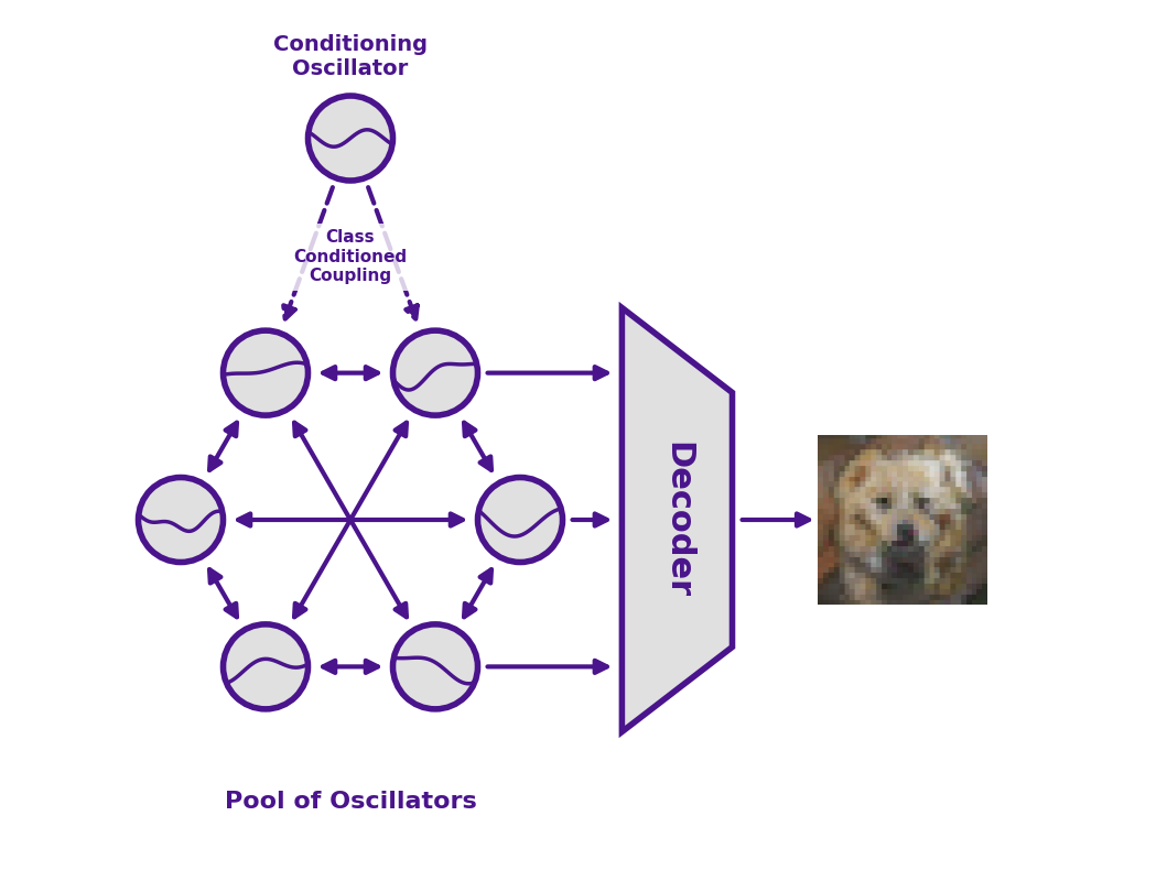
Figure 2: Coupled oscillators (with a unidirectional low rank class conditional matrix from the conditioning oscillators to the pool of oscillators) evolve through time under their trained coupling. Images are read-out at time, T, through a decoder to generate an image. Image distributions are generated by sampling the initial condition many times.
Model Architecture. Inference to generate an image with Un-0 follows five steps:
- Start from randomness. Set every oscillator's phase to a random angle
\theta_i \in [0, 2\pi). This random starting state is the seed, i.e., the counterpart to the noise a diffusion model or GAN samples. A different seed yields a different image. - Choose the class. A second, smaller group of oscillators drives the requested class (e.g., "daisy," or "volcano") and is coupled into the main population, biasing the main population toward arrangements associated with that class.
- Let physics execute. Release the system and let the oscillators pull on one another. The oscillators evolve away from their initial random start and settle toward a state dictated by their coupling.
- Take a snapshot. At a specified time, which we label
T, record the phase of every oscillator. That collection of final phases is a grid of numbers, a latent representation of the image. - Render. A conventional decoder (under 13% of the model's parameters) turns that latent representation into finished pixels.
Training changes only three things inside the model: 1) how the oscillators are coupled together (the matrix K), 2) each oscillator's natural frequency (\omega_i), and 3) the weights of the decoder. Together, the oscillators replace what would otherwise be a stack of conventional neural network layers.
Why this model architecture? We chose this model architecture to give the dynamics maximum flexibility to perform the computation. Specifically, the forward pass for training requires only 1) setting the coupling matrix, oscillator frequencies, and initial phases, 2) evolving the dynamics, and 3) reading the final image latents. This contrasts with other flavors of dynamical generation, such as diffusion [Sohl-Dickstein et al., 2015] and flow matching [Lipman et al., 2022], that explicitly guide the dynamics during training. However, the trade-off with our approach is that it requires a more complex loss that operates given only generated samples.
For more detail, we've placed a richer specification of the model in the Appendix.
How we built it
For both CIFAR-10 and ImageNet 64×64, we trained models of 3 different sizes.
CIFAR-10:
| Name | Oscillator count | Total trainable parameters | Oscillator parameters | Decoder parameters | Decoder fraction | FID@50k |
|---|---|---|---|---|---|---|
| Un-0.n1024 | 1024 | 1.29M | 1.13M | 0.16M | 12.24% | 11.01 |
| Un-0.n2048 | 2048 | 4.94M | 4.36M | 0.58M | 11.77% | 9.32 |
| Un-0.n4096 | 4096 | 19.43M | 17.11M | 2.33M | 11.96% | 8.76 |
ImageNet 64×64:
| Name | Oscillator count | Total trainable parameters | Oscillator parameters | Decoder parameters | Decoder fraction | FID@50k |
|---|---|---|---|---|---|---|
| Un-0.n6656 | 6656 | 57.17M | 50.96M | 6.21M | 10.86% | 8.41 |
| Un-0.n10240 | 10240 | 129.80M | 115.11M | 14.69M | 11.32% | 8.01 |
| Un-0.n16384 | 16384 | 322.44M | 284.84M | 37.61M | 11.66% | 6.74 |
Training. We trained the coupling matrix, oscillator frequencies, and decoder end-to-end on CIFAR-10 and ImageNet 64×64 using the recently proposed drifting loss (Deng et al., 2026) with a DINOv2 feature extractor [Oquab, Darcet, Moutakanni et al., 2024] and the AdamW optimizer. The model integrates the dynamics with an explicit Euler scheme.
Evaluation. We use standard evaluation methodology for these benchmarks. For CIFAR-10 models, we evaluated using 50k generated samples and compared to the reference CIFAR-10 statistics using the standard package and evaluation pipeline. For ImageNet 64×64 models, we evaluated using 50k generated samples and computed FID using the ADM evaluation suite.
Compute. We trained all CIFAR-10 models on 1xB200 GPU, and all ImageNet 64×64 models on 8xB200 GPUs. The largest CIFAR-10 model uses 20 B200 hours to train, and the largest ImageNet 64×64 model uses 640 B200 hours. The largest bottleneck in training is the computation of the drifting loss function, which requires the use of a conventional image feature extractor and is computed over many feature views.
Where Un-0 lands
We place Un-0 on a quality-vs-parameter-count curve against both conventional and unconventional models.
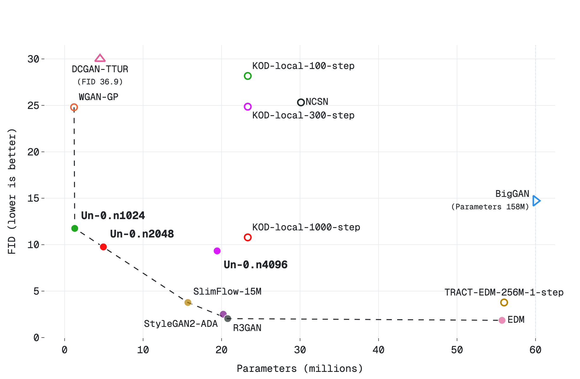
Figure 3a: Parameter count versus FID for CIFAR-10.
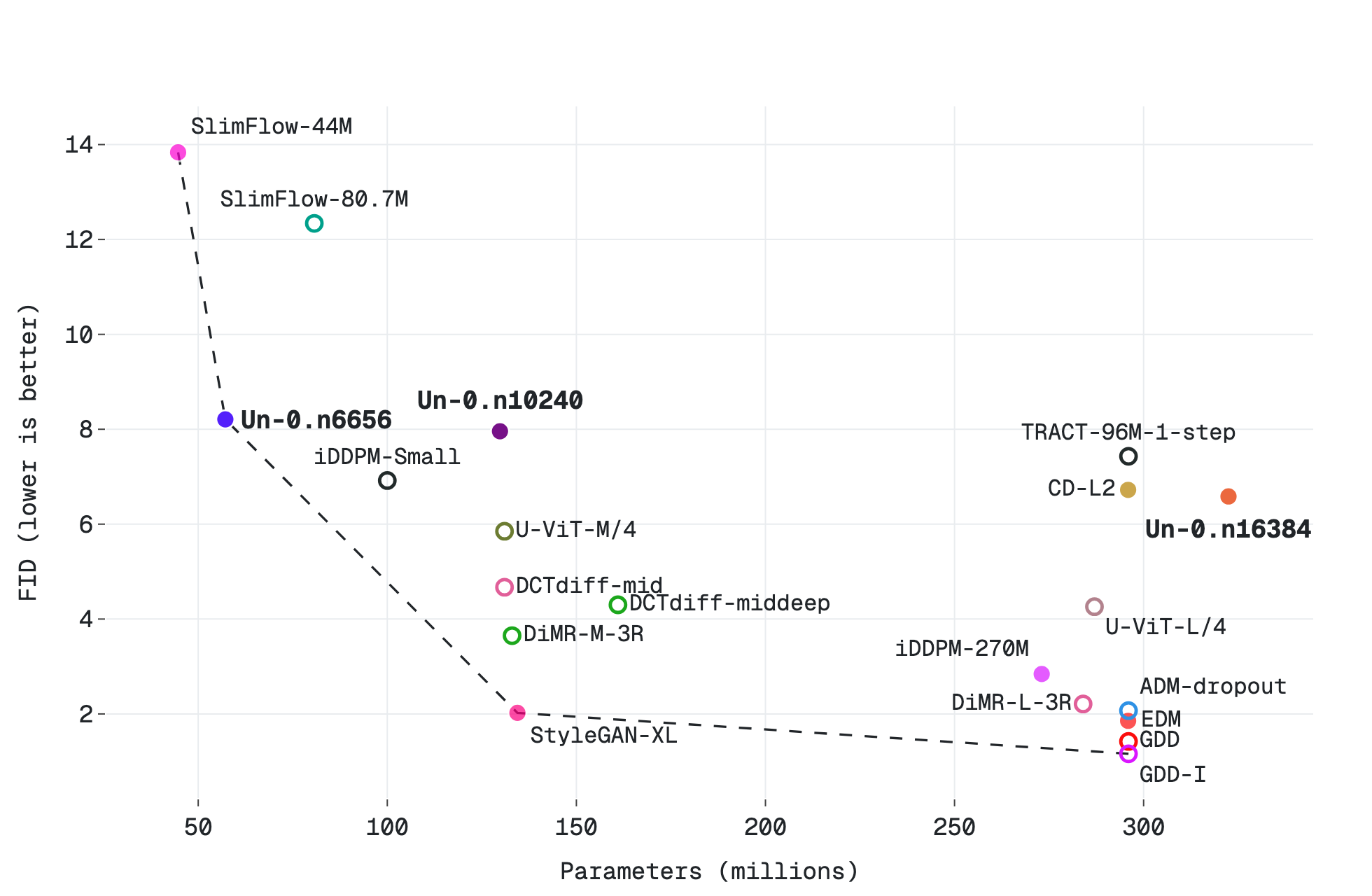
Figure 3b: Parameter count versus FID for ImageNet 64×64.
In the chart, solid dots are models we measured ourselves under the per-dataset identical FID-50k protocol. Hollow dots are published numbers we could not reproduce directly because code, checkpoints, or the exact evaluation setup were unavailable.
These published numbers should be read as reference points rather than strictly identical measurements, since evaluation protocols can differ across papers; for example, some results predate CleanFID and may use different Inception implementations or preprocessing details. When our reproduction closely matches the published result, we report our measured value; when a reproduction is clearly worse because of an unresolved setup mismatch, we defer to the published value and mark it as hollow.
For ImageNet 64×64, we specifically include models trained and evaluated at ImageNet 64×64 resolution, rather than results obtained by post-processing or downsampling from higher-resolution ImageNet models such as ImageNet 256×256. See the Reference section for the code and checkpoint links used for each model.
Discussion. Un-0’s quality sits alongside or above early conventional generators, such as NCSN, DCGAN-TTUR, WGAN-GP, BigGAN, iDDPM, CD, and TRACT (Song & Ermon, 2019; Heusel et al., 2017; Gulrajani et al., 2017; Brock et al., 2019; Nichol & Dhariwal, 2021; Song et al., 2023; Berthelot et al., 2023). Un-0 still trails later high-performing models such as EDM and GDD (Karras et al., 2022; Zheng & Yang, 2024). We view Un-0 as a promising first approach with quality that overlaps with that of several established image generation families when they were first introduced to the community.
For parameter count, Un-0 expands the Pareto frontier for small models amongst the comparison points we found. At larger sizes, Un-0 does not yet match state-of-the-art conventional baselines: quality keeps improving with scale, but more slowly than the conventional frontier. We interpret these results as the starting point of a new approach: the conventional methods we compare against took years of architectural and algorithmic refinement to scale from their own early days to where they are now. Improving how Un-0 scales through better learning algorithms, model architectures, and physical primitives is the next step.
Ablations
Un-0 is an unusual model in that we care not only about model quality, but we also want to attribute its behavior between the unconventional (oscillators) and conventional (decoder) components. If all the work is done by the conventional component, then the model doesn’t exploit the physical dynamics. To test this, we ablate the model to attribute responsibility and we find that the oscillators are doing useful computation.
We perform the following ablations. For each ablation, we performed a full learning rate sweep and chose the learning rate that led to the lowest FID for that specific ablation.
Decoder only. We trained the decoder in isolation, without the dynamics, by generating noise from the prior and pushing that noise through the decoder by itself, and optimizing the same loss as the full model. This baseline tells us how well the decoder can perform as a generative model in its own right, without the benefit of dynamics.
Reservoir. We train with the same loss as the full model, but fix the dynamical weights to their initial random initialization. This ablation checks if it is enough to merely use the dynamics as a random feature extractor, alternatively called a feature reservoir [Tanaka et al., 2019].
Time delta. For both the Un-0 and the reservoir, we vary the number of inference steps during training. With a single step of integration, the model behaves like a single layer in a typical neural network, or a dynamical system linearized about its initial condition. Increasing the number of integration steps increases the fidelity (and potential nonlinearity) of the underlying dynamical system. If the dynamics are truly performing non-trivial computation, we would expect greater fidelity and nonlinearity in the dynamics to lead to improved model performance. For the reservoir, we interpret the single integration step model as an unlearned random feature projection of the prior noise, and the multi-step model as a dynamical feature reservoir.
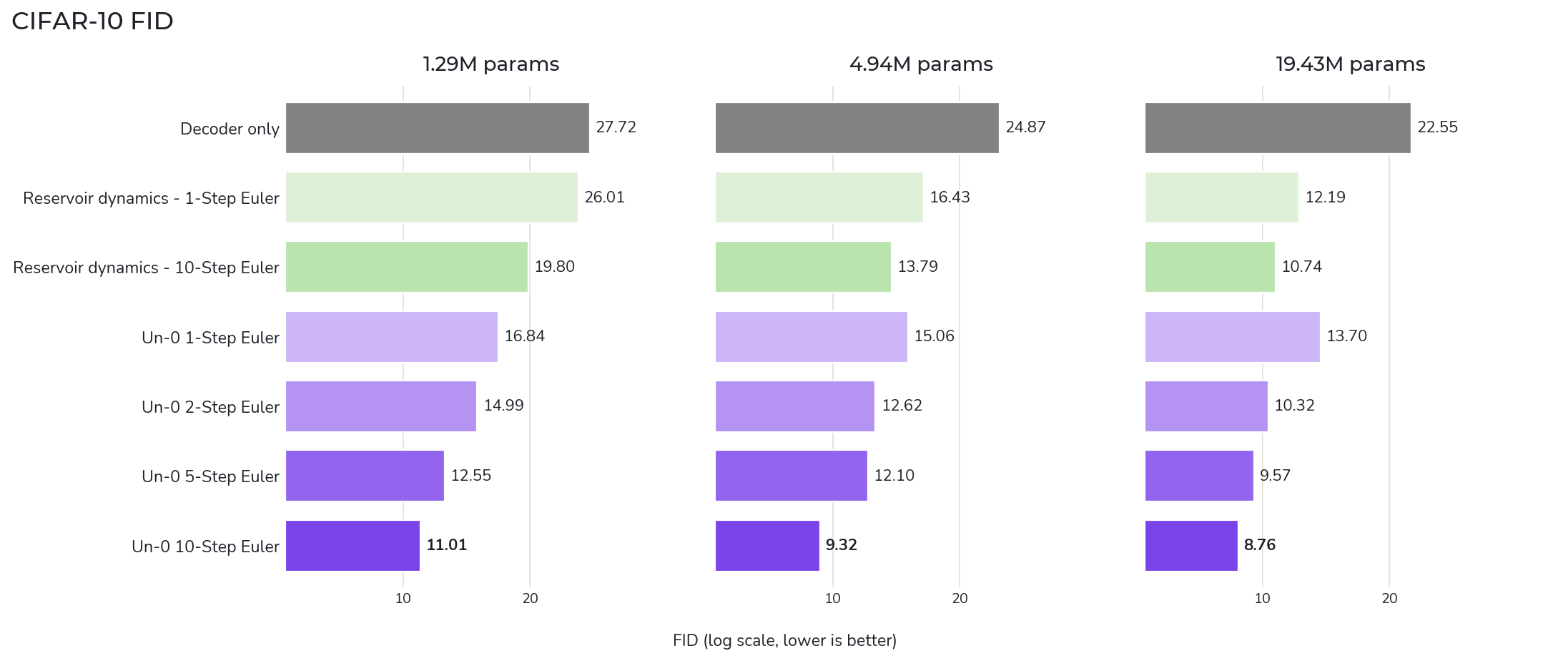
Figure 4a: Using the FID-50k protocol (where lower is better), we quantify the impact of our full suite of ablations ranging from removing dynamics (gray), freezing dynamics (green), and approximating dynamics (purple) on CIFAR-10 generation. We find that the trained dynamics are much more robust against decreasing size than the reservoir dynamics. Even at the largest model size, training the dynamics brings clear benefits to performance with long training times continuing to derive value.
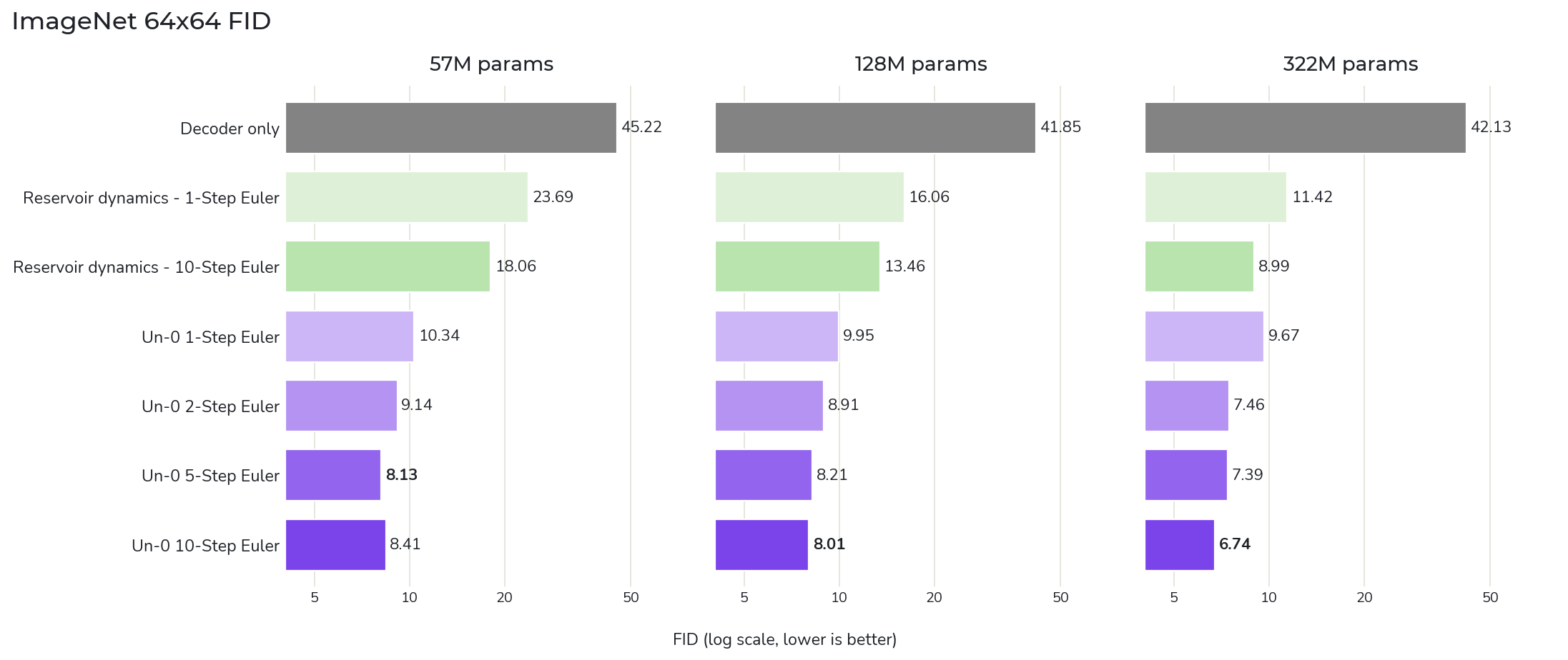
Figure 4b: Using the FID-50k protocol (where lower is better), we quantify the impact of our full suite of ablations ranging from removing dynamics (gray), freezing dynamics (green), and approximating dynamics (purple) on ImageNet 64×64 generation. We find that the trained dynamics are much more robust against decreasing size than the reservoir dynamics. Even at the largest model size, training the dynamics brings clear benefits to performance with long training times continuing to derive value.
Discussion. In both CIFAR-10 and ImageNet 64×64 models, we find that without the help of additional structure, the decoder struggles to map noise from the prior distribution to the target image distribution. However, even the small amount of structure provided by random Kuramoto dynamics, the reservoir produces a significant improvement, landing between the decoder only FID and the 1-step and 10-step reservoir model FIDs. We hypothesize that this is due to the random dynamics providing an input to the decoder that is more separable by the target class.
Interestingly, we see that the models with learned 1-step dynamics do not significantly outperform the reservoir dynamics on CIFAR-10; there does not appear to be much benefit to learning such a simple linearized dynamics in this setup. However, increasing the number of integration steps from 1 to 10 steps shows a clear trend of improving FID beyond the random dynamics baseline, with the best performing models being those with the most integration steps and learned dynamics.
We also checked if these learned dynamical models were simply overfitting to the specifics of the integrators used, and in the case of the models trained with 10 integration steps we see only a ~3% increase in FID when using many more integration steps or adaptive solvers.
These results together suggest that Un-0 is computing with the nonlinear dynamics beyond what is done by the other ablations.
What the dynamics are doing
Our ablations tell us that the dynamics matter; the natural next question is, how do the dynamics behave? The analyses below examine the behavior of the dynamics from several angles, building toward a hypothesis we explore at the end: the dynamics and the decoder play distinct roles, dynamics for diversity, decoder for image quality.
Separability. Our method does not train the full trajectory, but instead focuses on the T=1. By looking at the relative phase in decoder space at time T=1, we better understand how the dynamics serve the goal of improved image generation. To demonstrate class separability, we visualize 50 ImageNet 64×64 classes across the first three principal components to define a low dimensional projection.
Figure 5a: Integrating 1024 initial conditions out to T=1 across 50 ImageNet 64×64 classes reveals clear clustering in a low dimensional projection (Principal Components) of decoder space.
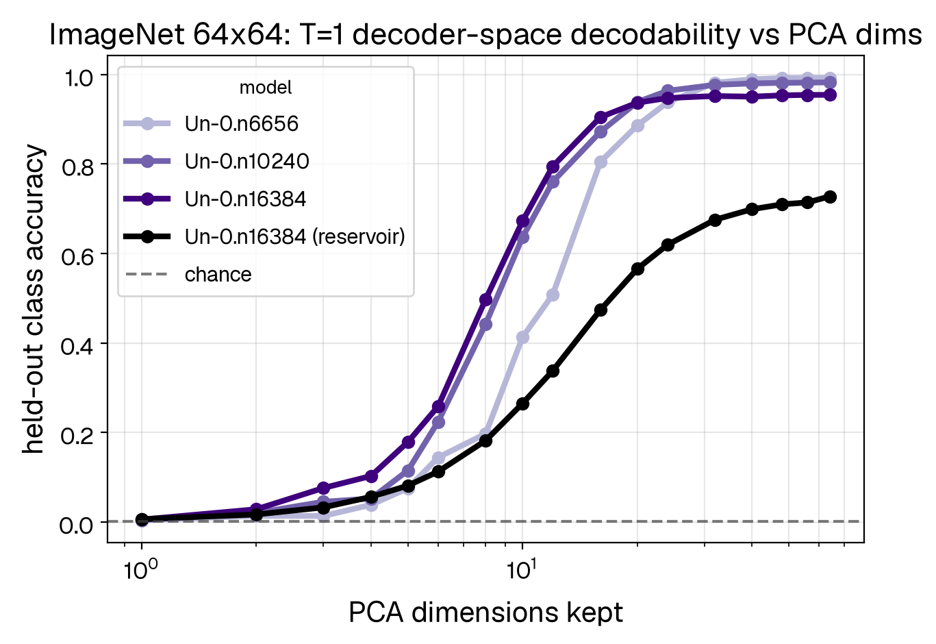
Figure 5b: By fitting an MLP from low dimensional coordinates to all 1k ImageNet 64×64 classes, we show that 32 dimensions in this low dimensional space is sufficient to classify 90%+ of the classes (top-1) in trained models while reservoirs show clear signatures of less separation in low dimensional space.
We find (see Figure 5a), that indeed trained networks exhibit a high degree of visual separability between classes at this critical timepoint. To check that this holds across all 1000 ImageNet 64×64 classes, we extend this to a decodability analysis designed to identify how much each set of low-dimensional coordinates encodes about the class (see Figure 5b). This combined analysis confirms that our objective acting at T = 1 drives separation at T = 1 in a low dimensional space relative to the effective decoder input dimensionality (e.g. 0.25% of the available dimensions).
Attractors. If we integrate our inference beyond T = 1, has the dynamics learned to achieve this clustering (see Figure 6) using fixed points or attractor manifolds? This would mean: given a random initial condition, the dynamics will flow toward one of many total fixed points (in rotating decoder space) stored within the dynamics.
Figure 6 (same as Figure 0): A sample of trajectories of Un-0.n4096 generations over time. Each line color has an associated box of similar color that denotes the class and generated images over time.
By plotting the dynamics (here CIFAR-10) of Un-0.n4096 in a low dimensional projection of decoder space (principal components of the covariance matrix), we observe the two phases of the dynamics. Phase 1: rapid separation of the class conditioned trajectories and phase 2: the slower refinement of the images. This notable second phase indicates the formation of class-conditional attractor manifolds.
Image Quality vs Diversity. Distributional measures such as FID combine single-sample image quality with image diversity/coverage [Sajjadi et al., 2018; Kynkäänniemi et al., 2019]. This means that FID can be limited by either image precision (image quality — as seen in screenshots) or recall (distributional coverage in generation).
For example, the FID score for a model that maps all generations to a single cat image would be poor due to low diversity (low recall) even if that image of the cat is of the highest quality (high precision). Therefore, to complement FID, we leverage precision and recall as measurable proxies for image quality and diversity [Kynkäänniemi et al., 2019; Dhariwal & Nichol, 2021].
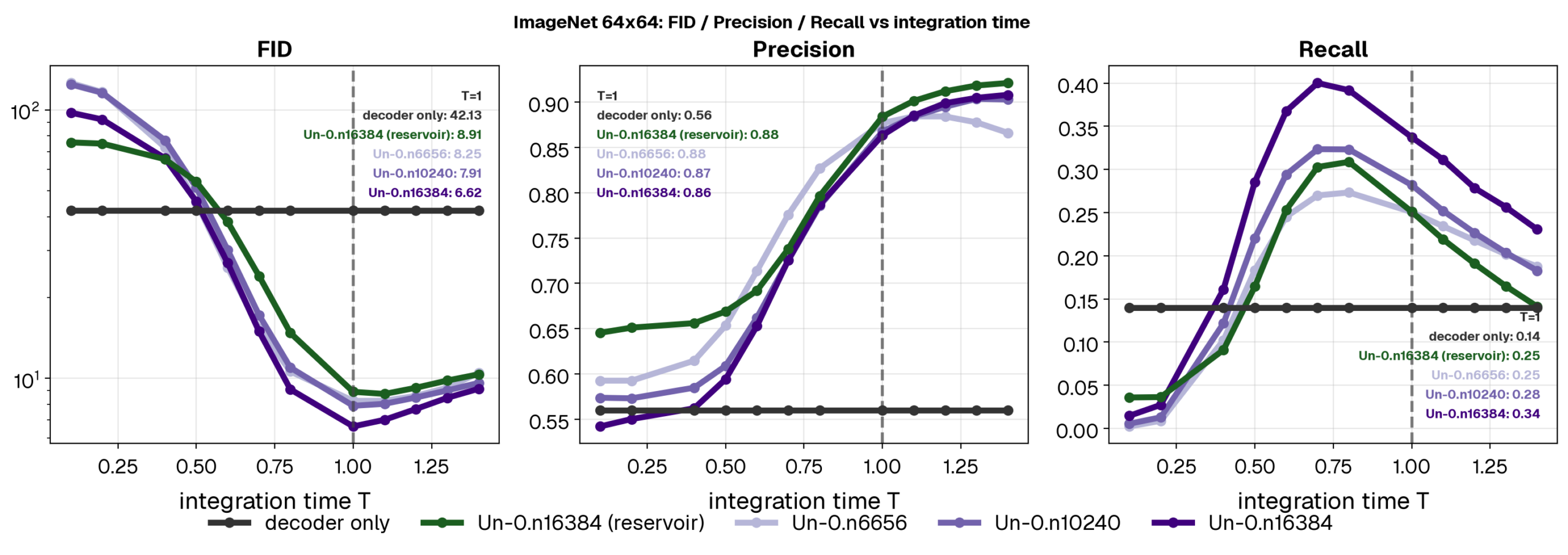
Figure 7: The model class generates images through time. Here, we plot three metrics of performance: a) FID (lower is better) between the samples and the data, b) Precision (higher is better) as a proxy of image quality, and c) recall (higher is better) as a proxy for image diversity. Notice that FID quickly drops as the dynamics play out illustrating the central role the dynamics (whether training or not) plays in shaping the distribution. We show that dynamics improves our images by ~2.5 at the largest system size and since we are in the recall limited regime, this improvement is predominantly attributable to measurable increases in the recall peak and, by extension, the recall at T=1 (+0.10 recall).
Watching the time dynamics of image generation, our trained models start off randomly and in bulk generate poor quality images which are highly diverse (low precision, high recall). As time progresses, the dynamics of our Kuramoto system pulls diverse initial conditions to states consistent with dogs, cats, and mushrooms (high precision + intermediate recall/diversity). In an untrained reservoir, the dynamics continue reducing recall dramatically. As time progresses FID becomes limited not by image quality but image diversity. Strikingly, a trained network measurably increases this diversity of state across time meaning that the dynamics begin to align with the class manifold. Indeed our ablation studies show this as well in low final recall of Decoder only and reservoirs relative to trained Kuramoto dynamics.
This leads to the simplified cartoon of the hypothesis we set out to explore: this hybrid system factorizes responsibilities such that the dynamics of Kuramoto preserve diversity (giving rise to generalization of performance across inference time) and the conventional decoder serves the role of image quality generator. On the horizon, we envision fully unconventional means to generating diverse samples of high quality images amenable to the physical dynamics on a chip.
Conclusion
Un-0’s quality matches where today’s leading generative methods began. Conventional generators are still stronger on absolute quality and parameter efficiency — closing that gap with new algorithms and model architectures is the work ahead.
Taken together, Un-0’s system of coupled Kuramoto oscillators offers the promise of learning with physical dynamics at a scale that’s beyond what has been done before. Un-0 points in the direction of the opportunity for a new computer that exploits physics to achieve our top-line goal of energy efficiency: iso-quality, joules per inference for modern AI.
Try it, and join the mission
We’re releasing:
- Model weights of the Kuramoto models, for both CIFAR-10 and ImageNet.
- Training scripts to reproduce our training results and extend them for custom models.
- Ablation scripts — the full suite — so anyone can run the same controls on their own dynamics.
Please check out GitHub for details.
Stay tuned as we and others close the gap with new algorithms, models, and physical primitives. We as a community are at the beginning of the beginning for unconventional AI systems. It is a grand, full-stack challenge to achieve 1000x efficiency improvement in modern AI, but the community’s results offer a promising path forward together.
If you build physics-based models — or anything with a dynamical core — plug them into our Un-0 scaffold, train them, and see where they land. If this is the kind of question you want to work on with us: come work with us, reach out as a collaborator, and/or follow what we do next.
References
- Shiqi Chen, Yuhang Li, Yuntian Wang, Hanlong Chen, Aydogan Ozcan. “Optical generative models.” Nature 2025.
- Ilker Oguz, Niyazi Ulas Dinc, Mustafa Yildirim, Junjie Ke, Innfarn Yoo, Qifei Wang, Feng Yang, Christophe Moser, Demetri Psaltis. “Optical Diffusion Models for Image Generation.” NeurIPS 2024.
- Tiankuang Zhou, Yizhou Jiang, Zhihao Xu, Zhiwei Xue, Lu Fang. “Hundred-layer photonic deep learning.” Nature Communications 2025.
- Jiaqi Chu, Heiner Kremer, Fabian Falck, Grace Brennan, Burcu Canakci, James Clegg, Daniel Cletheroe, Doug Kelly, Christos Gkantsidis, Michael S. Hansen, Paul Jeha, Kirill P. Kalinin, Jim Kleewein, Babak Rahmani, Saravan Rajmohan, Victor Rühle, Jannes Gladrow, Francesca Parmigiani, Hitesh Ballani. “Analog Diffusion Models.” 2026.
- Andraž Jelinčič, Owen Lockwood, Akhil Garlapati, Guillaume Verdon, Trevor McCourt. “An efficient probabilistic hardware architecture for diffusion-like models.” 2025.
- Zhihao Xu, Tiankuang Zhou, Muzhou Ma, ChenChen Deng, Qionghai Dai, Lu Fang. “Large-scale photonic chiplet Taichi empowers 160-TOPS/W artificial general intelligence.” Science 2024.
- Stephen Whitelam. “Generative thermodynamic computing.” Physical Review Letters 136, 037101, 2026.
- Cyrill Bösch, Geoffrey Roeder, Marc Serra-Garcia, Ryan P. Adams. “Local Learning Rules for Out-of-Equilibrium Physical Generative Models.” arXiv:2506.19136, 2025.
- Carver Mead. “Neuromorphic Electronic Systems.” Proceedings of the IEEE 78(10):1629–1636, 1990.
- Patrick J. Coles, Collin Szczepanski, Denis Melanson, Kaelan Donatella, Antonio J. Martinez, Faris Sbahi. “Thermodynamic AI and the fluctuation frontier.” arXiv:2302.06584, 2023.
- Andraž Jelinčič, Owen Lockwood, Akhil Garlapati, Peter Schillinger, Isaac Chuang, Guillaume Verdon, Trevor McCourt. “An efficient probabilistic hardware architecture for diffusion-like models.” arXiv:2510.23972, 2025.
- Sohl-Dickstein, Jascha, et al. “Deep unsupervised learning using nonequilibrium thermodynamics.” ICML, 2015.
- Lipman, Yaron, Ricky TQ Chen, Heli Ben-Hamu, Maximilian Nickel, and Matt Le. “Flow matching for generative modeling.” 2022.
- Jonathan Ho, Ajay Jain, Pieter Abbeel. “Denoising Diffusion Probabilistic Models.” NeurIPS 2020.
- Yang Song, Stefano Ermon. “Generative Modeling by Estimating Gradients of the Data Distribution.” NeurIPS 2019.
- Oquab, Maxime, Timothée Darcet, Théo Moutakanni, Huy Vo, Marc Szafraniec, Vasil Khalidov, Pierre Fernandez et al. “DINOv2: Learning robust visual features without supervision.” TMLR 2024.
- Yang Song, Stefano Ermon. “Improved Techniques for Training Score-Based Generative Models.” NeurIPS 2020.
- Yang Song, Prafulla Dhariwal, Mark Chen, Ilya Sutskever. “Consistency Models.” ICML 2023. arXiv:2303.01469
- Tero Karras, Miika Aittala, Timo Aila, Samuli Laine. “Elucidating the Design Space of Diffusion-Based Generative Models” (EDM). NeurIPS 2022. arXiv:2206.00364
- Alex Nichol, Prafulla Dhariwal. “Improved Denoising Diffusion Probabilistic Models.” ICML 2021. arXiv:2102.09672
- Mingyang Deng, He Li, Tianhong Li, Yilun Du, Kaiming He. “Generative Modeling via Drifting.” 2026. arXiv:2602.04770
- J. Deng, W. Dong, R. Socher, L.-J. Li, K. Li, and L. Fei-Fei. “ImageNet: A large-scale hierarchical image database.” CVPR 2009.
- Krizhevsky, Alex, and Geoffrey Hinton. “Learning multiple layers of features from tiny images.” 2009.
- Sajjadi, Mehdi SM, Olivier Bachem, Mario Lucic, Olivier Bousquet, and Sylvain Gelly. “Assessing generative models via precision and recall.” Advances in Neural Information Processing Systems 31 (2018).
- Kynkäänniemi, Tuomas, Tero Karras, Samuli Laine, Jaakko Lehtinen, and Timo Aila. “Improved precision and recall metric for assessing generative models.” Advances in Neural Information Processing Systems 32 (2019).
- Charles M. Gray, Peter König, Andreas K. Engel, Wolf Singer. “Oscillatory responses in cat visual cortex exhibit inter-columnar synchronization which reflects global stimulus properties.” Nature 338(6213):334–337, 1989. doi:10.1038/338334a0
- György Buzsáki. Rhythms of the Brain. Oxford University Press, 2006. OUP
- John J. Hopfield. “Neural networks and physical systems with emergent collective computational abilities.” PNAS 79(8):2554–2558, 1982. pnas.org
- Herbert Jaeger. “The ‘echo state’ approach to analysing and training recurrent neural networks.” GMD Report 148, 2001. PDF
- Wolfgang Maass, Thomas Natschläger, Henry Markram. “Real-time computing without stable states.” Neural Computation 14(11):2531–2560, 2002. MIT Press
- Sam Greydanus, Misko Dzamba, Jason Yosinski. “Hamiltonian Neural Networks.” NeurIPS 2019. arXiv:1906.01563
- Ramin Hasani, Mathias Lechner, Alexander Amini, Daniela Rus, Radu Grosu. “Liquid Time-constant Networks.” AAAI 2021. arXiv:2006.04439
- Takeru Miyato, Sindy Löwe, Andreas Geiger, Max Welling. “Artificial Kuramoto Oscillatory Neurons.” ICLR 2025. arXiv:2410.13821
- Yue Song, T. Anderson Keller, Sevan Brodjian, Takeru Miyato, Yisong Yue, Pietro Perona, Max Welling. “Kuramoto Orientation Diffusion Models.” NeurIPS, 2025. arXiv:2509.15328
- T. Anderson Keller, Max Welling. “Neural Wave Machines: Learning Spatiotemporally Structured Representations with Locally Coupled Oscillatory Recurrent Neural Networks.” ICML 2023. PMLR v202
- Tanaka, Gouhei, Toshiyuki Yamane, Jean Benoit Héroux, Ryosho Nakane, Naoki Kanazawa, Seiji Takeda, Hidetoshi Numata, Daiju Nakano, and Akira Hirose. “Recent advances in physical reservoir computing: A review.” Neural Networks 115 (2019): 100–123. arXiv:1808.04962
- Fries, Pascal. “Rhythms for Cognition: Communication through Coherence.” Neuron 88, 220–235 (2015). neuron
- Ermentrout, Bard. “Type I Membranes, Phase Resetting Curves, and Synchrony.” Neural Computation 8, 979–1001 (1996). doi:10.1162/neco.1996.8.5.979
- Ermentrout, Bard, and Terman, David. Mathematical Foundations of Neuroscience, Interdisciplinary Applied Mathematics. Springer, New York, NY (2010). doi:10.1007/978-0-387-87708-2
- Kuramoto, Yoshiki. “Self-entrainment of a population of coupled non-linear oscillators, in: Mathematical Problems in Theoretical Physics.” pp. 420–422 (1975). doi:10.1007/BFb0013365
- Winfree, Arthur T. “Biological rhythms and the behavior of populations of coupled oscillators.” J Theor Biol 16, 15–42 (1967). doi:10.1016/0022-5193(67)90051-3
- Prafulla Dhariwal, Alex Nichol. “Diffusion Models Beat GANs on Image Synthesis.” NeurIPS 2021. arXiv:2105.05233
Appendix
Formal Model Specification. The model is a class-conditional implicit generative model with initial phases sampled from a uniform distribution from 0 to 2\pi. The initial random phases evolve according to the ODE above for a fixed amount of time T. To incorporate class conditioning, the model couples a large system of N shared oscillators to a separate smaller array of N_c conditioning oscillators with uni-directional, class conditional couplings:
\dot{\theta}_i = \omega_i + \sum_{j=1}^{N} K_{ij}\,\sin(\theta_j - \theta_i) + \sum_{k=1}^{N_c}\tilde{K}^{(c)}_{ki}\sin(\phi_k - \theta_i) \qquad i = 1, \dots, N
Here, \tilde{K}^{(c)}\in\mathbb{R}^{N_c\times N} is a class-specific coupling matrix representing the class-specific coupling weights to the conditioning oscillators. The conditioning oscillators evolve according to the Kuramoto dynamics
\dot{\phi}_i = \nu_i + \sum_{j=1}^{N_c} C_{ij}\,\sin(\phi_j - \phi_i), \qquad i = 1, \dots, N_c
For conditioning oscillators \phi and couplings C_{ij}\in\mathbb{R}^{N_c\times N_c}. At T the phases are read out and converted to euclidean space via a sin/cos decode:
x_i,\ y_i = \cos(\theta_i - \theta_{ref}),\ \sin(\theta_i - \theta_{ref})
Where \theta_{ref} is a reference phase: the mean of all phases \theta_{ref} = \frac{1}{N}\sum_{i=1}^N \theta_i for CIFAR-10 models and the phase of the first oscillator \theta_{ref} = \theta_0 for ImageNet 64x64 models. The decoded x_i, y_i features are reshaped into an image-like latent grid of shape (C_l, h_l, w_l) and fed into an upsampling decoder which iterates 2x spatial upsampling + 2x 3x3 convolution blocks to convert the image latents into the final (3, H, W) image. The decoder upsamples by a factor of 8 for the CIFAR-10 models, and a factor of 16 for the ImageNet 64x64 models. In each model, the decoder accounts for less than 15% of the total parameters. Note the oscillator array is initially unstructured; we do not include any explicit task-specific inductive biases in the couplings.
FID x Parameter Figure reproduction
CIFAR-10
| Model handle | Paper | Resource |
|---|---|---|
| BigGAN | Brock et al., 2019 | code |
| DCGAN-TTUR | Heusel et al., 2017 | code |
| DCTdiff-mid | Ning et al., 2024 | code |
| EDM | Karras et al., 2022 | code, checkpoint |
| KOD-local-100-step | Song et al., 2025 | code |
| KOD-local-300-step | Song et al., 2025 | code |
| KOD-local-1000-step | Song et al., 2025 | code |
| NCSN | Song & Ermon, 2019 | code |
| R3GAN | Huang et al., 2025 | code, checkpoint |
| SlimFlow 15M | Zhu et al., 2024 | code, checkpoint |
| StyleGAN2-ADA | Karras et al., 2020 | code, checkpoint |
| TRACT-EDM-256M-1-step | Berthelot et al., 2023 | |
| WGAN-GP | Gulrajani et al., 2017 |
ImageNet 64×64
| Model handle | Paper | Resource |
|---|---|---|
| ADM-dropout | Dhariwal and Nichol, 2021 | code, checkpoint |
| CD L2 | Song et al., 2023 | code, checkpoint |
| DCTdiff-small | Ning et al., 2024 | code, checkpoint |
| DCTdiff-mid | Ning et al., 2024 | code, checkpoint |
| DCTdiff-middeep | Ning et al., 2024 | code, checkpoint |
| DiMR-L 3R | Liu et al., 2024 | code |
| DiMR-M 3R | Liu et al., 2024 | code |
| EDM | Karras et al., 2022 | code, checkpoint |
| EDM2-L | Karras et al., 2024 | |
| GDD | Zheng and Yang, 2024 | |
| GDD-I | Zheng and Yang, 2024 | |
| iDDPM 270M | Nichol and Dhariwal, 2021 | code, checkpoint |
| iDDPM Small | Nichol and Dhariwal, 2021 | code |
| SlimFlow 44M | Zhu et al., 2024 | code, checkpoint |
| SlimFlow 80.7M | Zhu et al., 2024 | code |
| StyleGAN-XL | Sauer et al., 2022 | code, checkpoint |
| TRACT-96M-1-step | Berthelot et al., 2023 | |
| U-ViT-L/4 | Bao et al., 2023 | code |
| U-ViT-M/4 | Bao et al., 2023 | code |