

Aug 13, 2026
Research
Less is More: Scaling Dynamics with Sparsity
TL;DR – In the original Un-0 model architecture, the number of connections between oscillators — and trainable parameters — increases precipitously as the oscillator count grows since the oscillators are connected all-to-all. Such architectures are challenging to implement at scale in hardware. We explore two methods for introducing sparsity into the model architecture to reduce the number of interactions and enhance scaling, eliminating 50%-98.4% of the interactions. Surprisingly, we also find both forms of sparsity improve the performance/trainability of this class of models. On ImageNet 64×64, sparse architectures achieve an FID of 7.15, improving upon the densely connected Un-0 baseline with 6657 oscillators by ~1.9 FID. This improvement holds across multiple workloads including CIFAR-10 generation and MNIST1D classification tasks.
In our Un-0 model release blog post, every oscillator is connected, or coupled, to every other oscillator with a programmable weight. This creates scalability issues: as the oscillator count (N) increases, the number of connections (N^2) grows quadratically. For a thousand oscillators, this would translate to a million couplings; for a million oscillators, one trillion couplings. This relationship places steep design constraints on the hardware as the system scales, requiring increasingly large numbers of programmable interactions between every possible pair of oscillators. In this article, we demonstrate that this scaling trend can be tamed by sparsifying the connections between oscillators, and explore two methods for doing so. By eliminating large numbers of connections, we reduce the number of parameters in the model and relax connectivity requirements imposed on the hardware, simultaneously reducing data movement and simplifying hardware design. We also find that these methods have the unexpected benefit of enhancing the model’s trainability, improving training outcomes at larger system sizes.
0. Refresher on ML with Coupled Oscillators
All model architectures in this blog perform computation with large networks of coupled oscillators, commonly modeled as Kuramoto oscillators. Concretely, each oscillator's motion follows a single rule, applied continuously over time: it rotates at its own natural frequency, nudged by the pull of every other oscillator. The following ordinary differential equation (ODE) describes the evolution of the oscillators over time:
\dot{\theta}_i = \omega_i + \sum_{j=1}^{N} K_{ij}\,\sin(\theta_j - \theta_i), \qquad i = 1, \dots, N
Each oscillator i carries a phase \theta_i \in [0,2\pi), and \omega_i is its natural frequency. The coupling matrix K_{ij} specifies the coupling strength that sets how strongly oscillator i pulls j toward or away from alignment. During training the coupling matrix K and the frequencies \omega are learned; these are the parameters of the physical system. In this article, we explore two strategies for sparsifying the coupling matrix K to reduce the number of parameters and relax connectivity requirements.
1. Two Sparsification Strategies: Random Sparsity and Modularity
 |
Random Sparse Coupling Matrix |
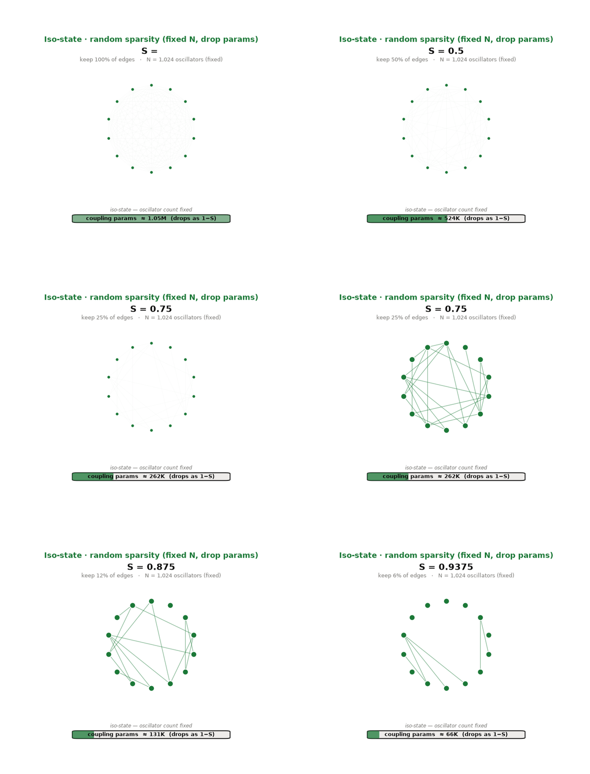
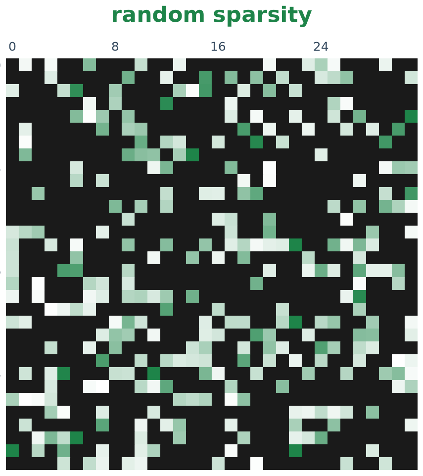
In random sparsity, a fraction of connections are randomly deleted. Before training, each potential coupling is randomly deleted with a probability (s) referred to as the sparsity of the architecture. A random sparse N-oscillator network will have (1-s) \cdot N^2 connections. At high levels of sparsity, very few connections are retained. A network with 99% sparsity (s=0.99) only keeps 1% of the couplings from the original all-to-all network. In these sparse networks, only subsets of oscillators need to be connected together, removing the need for all-to-all connectivity.
The neuroAI community has studied RNNs with fixed sparsity masks (Turcu & Abbott, 2022; Xie et al., 2025; Fruengel, 2025; Caranzano et al., 2025; Jiao et al., 2026; see the appendix). In contrast to work using dynamic masks in feedforward networks (LeCun et al., 1989; Han et al., 2015; Frankle et al., 2019; Liebenwein et al., 2021), these studies treat unstructured/random sparsity as a biophysically motivated constraint with important implications for dynamics such as generalization (Jiao et al., 2026), and slow transitions to chaos (Xie et al., 2025). More recently these phenomena have been combined to demonstrate improved sample efficiency in sparse networks (Bellec et al., 2018; Fruengel et al., 2025). Our work leverages a similar sparsity strategy to build more scalable physics-based architectures on larger scale image generation tasks.
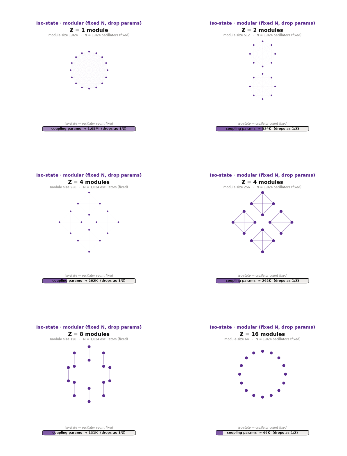
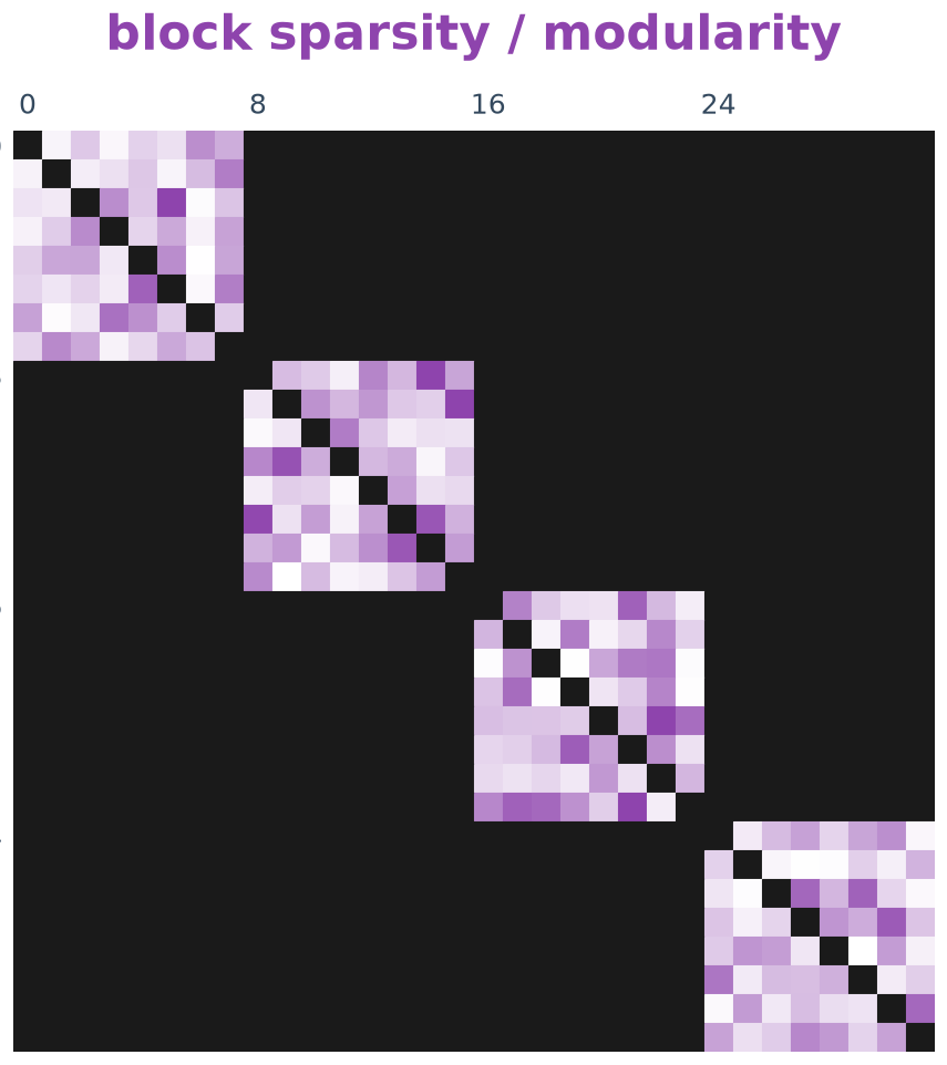
Figure 2: Increasing the number of modules at fixed number of oscillators. |
Modular Coupling Matrix |
For structured sparsity, we consider modular sparsity: the oscillators are partitioned into roughly equally sized groups called modules. In this work, oscillators are connected all-to-all within each module, but the modules themselves are not connected. For a modular N oscillator network partitioned into Z modules, the model has \frac {N^2} Z coupling parameters. For a network with 32 modules, only 3% of couplings from the original all-to-all network are kept. Similar to random sparsity, only small subsets of oscillators need to be connected all-to-all, reducing connectivity requirements. The sparsity of a modular architecture is simply 1 - 1/Z, where 1/Z is the fraction of parameters kept.
Structured sparsity, specifically modular sparsity has traditionally been used to achieve computational efficiency (Grey et al., 2017; Zhou et al., 2021). However, motivated by observations of modularity in the brain (Litwin-Kumar et al., 2012; Hizanidis et al., 2016; Semedo et al., 2019), the community has explored the computational power of modular networks (Kozachkov et al., 2022; Kuśmierz et al., 2025) and recurrent independent mechanisms (Goyal et al., 2021). Similarly, our work shows that static modular sparsity in recurrent populations of oscillators can improve performance though we target larger computational tasks such as image generation.
(For a more comprehensive discussion of this literature, please see "Related Work" in the Appendix.)
2. Un-0 with Random Sparsity and Modularity
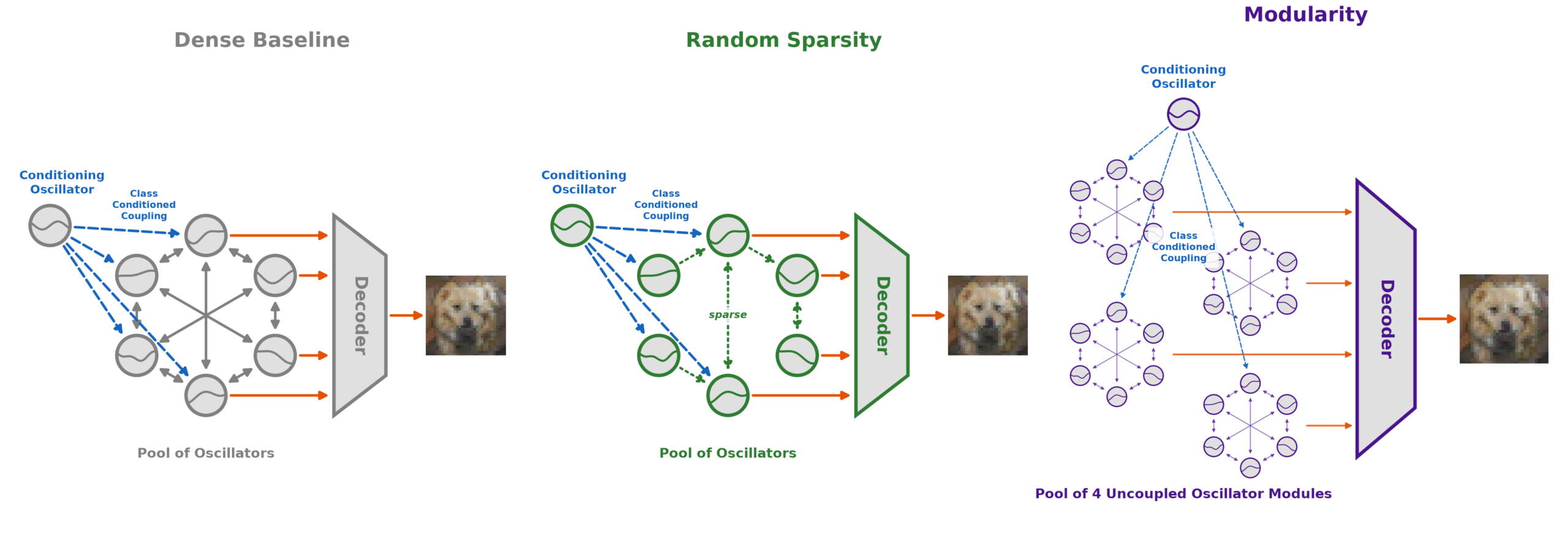 Figure 3: We study our dense baseline (gray) compared to two sparse variants of the Un-0.n1024 model: 1) random sparsity (green) and modularity (purple).
We apply both modular and random sparsity to Un-0, a family of oscillator-based models that target image generation tasks. The original architecture has a dense all-to-all oscillator coupling scheme; in this blog we train Un-0 with random sparsity and modular sparsity on both CIFAR-10 and ImageNet 64×64. Figure 3 diagrams the original (left), random sparse (middle), and modular (right) architectures under study. Refer to the appendix for a detailed list of modifications.
CIFAR-10 Generation: For CIFAR-10 we compare against an all-to-all connected ~1032 oscillator baseline (1024 main pool oscillators + 8 conditioning oscillators) with 1.22M parameters. For both sparse and modular configurations, we build iso-oscillator and iso-coupling models, which match the oscillator pool size and the pool coupling count at different levels of sparsity:
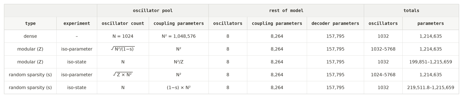 Table 1: We compare the closed-form solutions for our four experiments under fixed decoder capacity by combining the scaling method (iso-state vs iso-parameter-count) and the form of sparsity (random vs modularity).
For all configurations, the decoder size and conditioning oscillator count are fixed. Together, these fixed-decoder-size configurations allow us to explore how the model performs as we increase sparsity to reduce parameter counts (in the iso-oscillator case), and to increase the amount of oscillator state without changing the number of parameters (iso-parameter).
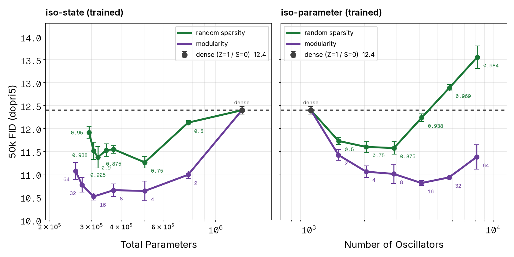 Figure 4: Across both forms of sparsity comparing iso-state scaling (left), and iso-parameter count scaling (right), we find broad regimes of sparsity/modularity that exhibit improved performance over our dense baseline Un-0.n1024. For discussion of the mechanism see sections.
In the iso-state experiments (left, Figure 4) both random sparsity and modularity deliver FID improvements over the fully dense baseline at reduced parameter counts. In the iso-parameter-count experiment (right, Figure 4) both random sparsity and modularity achieve FID reductions when given more oscillators, even if more parameters are not added to the model and these oscillators are not densely connected.
Importantly, we note that above a critical sparsity (which is different for modularity vs random sparsity) more sparsity is detrimental. In the following sections we investigate the role of dynamics diversity as a mechanism for the initial improvement, and loss of communication as the mechanism for high sparsity failure.
ImageNet 64×64 Generation: For ImageNet 64×64, we compare against the all-to-all connected 6656 oscillator baseline with 57M parameters from the Un-0 blog. We evaluate both 75% sparse and 16-module implementations of the same model:

Table 2: We conduct two iso-state scaling experiments for both random sparsity and modularity on ImageNet 64×64.
We observe a ~1.9 FID improvement over baseline when training the modular variant of Un-0.n6657 (Z=16) which measurably advances the smallest (parameter count) model in the Un-0 family for ImageNet 64×64. These experiments lend support to the hypothesis that modularity and random sparsity can further both hardware and model performance at scale.
3. Ablation: Dynamics and Training
We repeat the ablation from the (dense) Un-0 release, but with random sparsity and modularity. The dense ablation is included for reference (left). As we can see the same general trends hold for the sparse architectures — the reservoir does significantly worse than the trained dynamics, and the trained dynamics get progressively better FIDs as the number of time steps increases. These observations suggest that (1) training the model is integral to achieving the observed FID and (2) the dynamics contribute to the performance of the model.
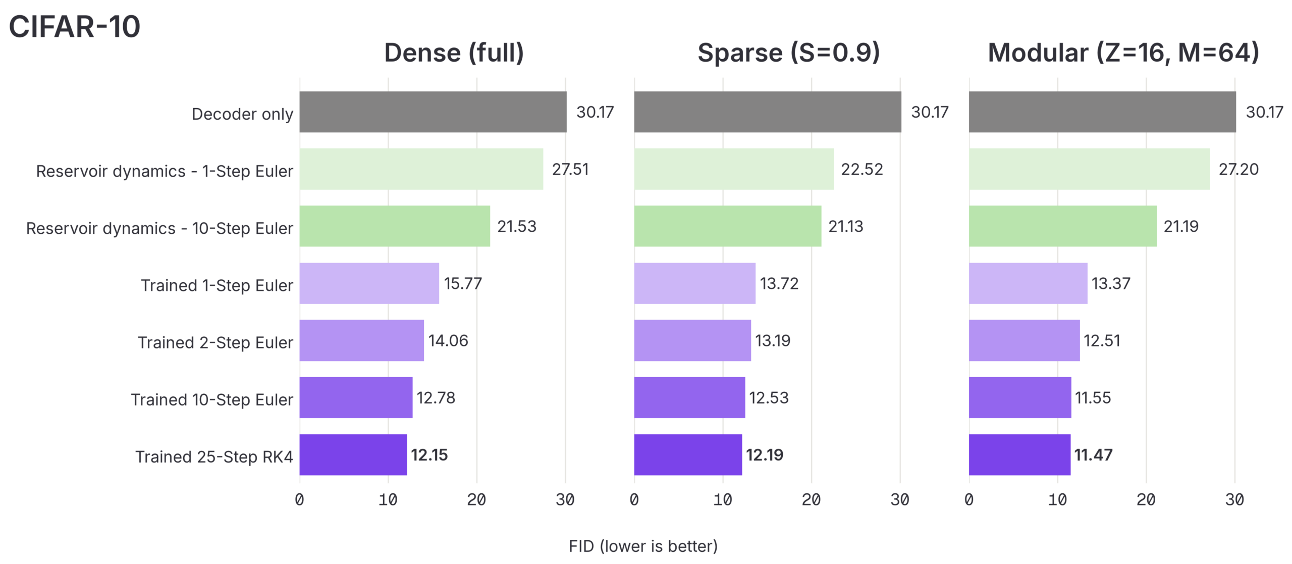 Figure 5: We apply the Un-0 release ablation suite across three of our CIFAR-10 iso-state checkpoints: dense (left), random sparsity (middle) and modular sparsity (right). The gap between the decoder-only, reservoir, and across integration fidelity suggests that dynamics remain important even in the sparse limit.
Across these ablations (see Figure 5 and 6), we continue to see evidence that 1) dynamics is better than decoder-only, 2) training the dynamics improves over reservoir dynamics, and 3) more steps of integration provides more benefit. We interpret these results as support for the thesis: sparsity helps Un-0-like models through training.
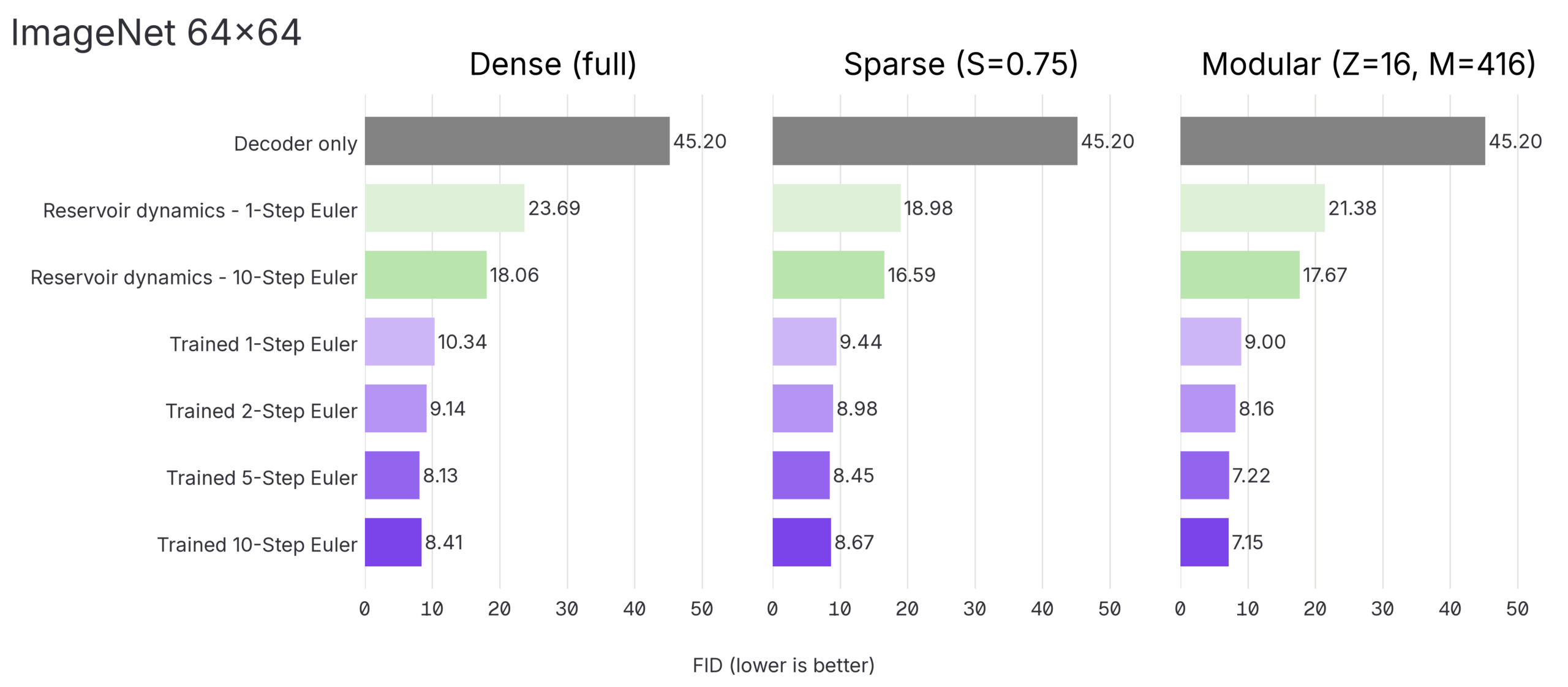 Figure 6: We apply the Un-0 release ablation suite across three of our ImageNet 64×64 checkpoints: dense (left), random sparsity (middle) and modular sparsity (right). The gap between the decoder-only, reservoir, and across integration fidelity suggests that dynamics remain important even in the sparse limit.
4. Analysis of Modular Un-0
Watching the dynamics. Because the modular architecture is built from a handful of disconnected modules, it is amenable to being inspected and reverse engineered. The below visualization simulates the oscillator state for each module (Fig 7A), the decoder state (Fig 7B), the decoded image (Fig 7C), and the class probability over time (Fig 7D).
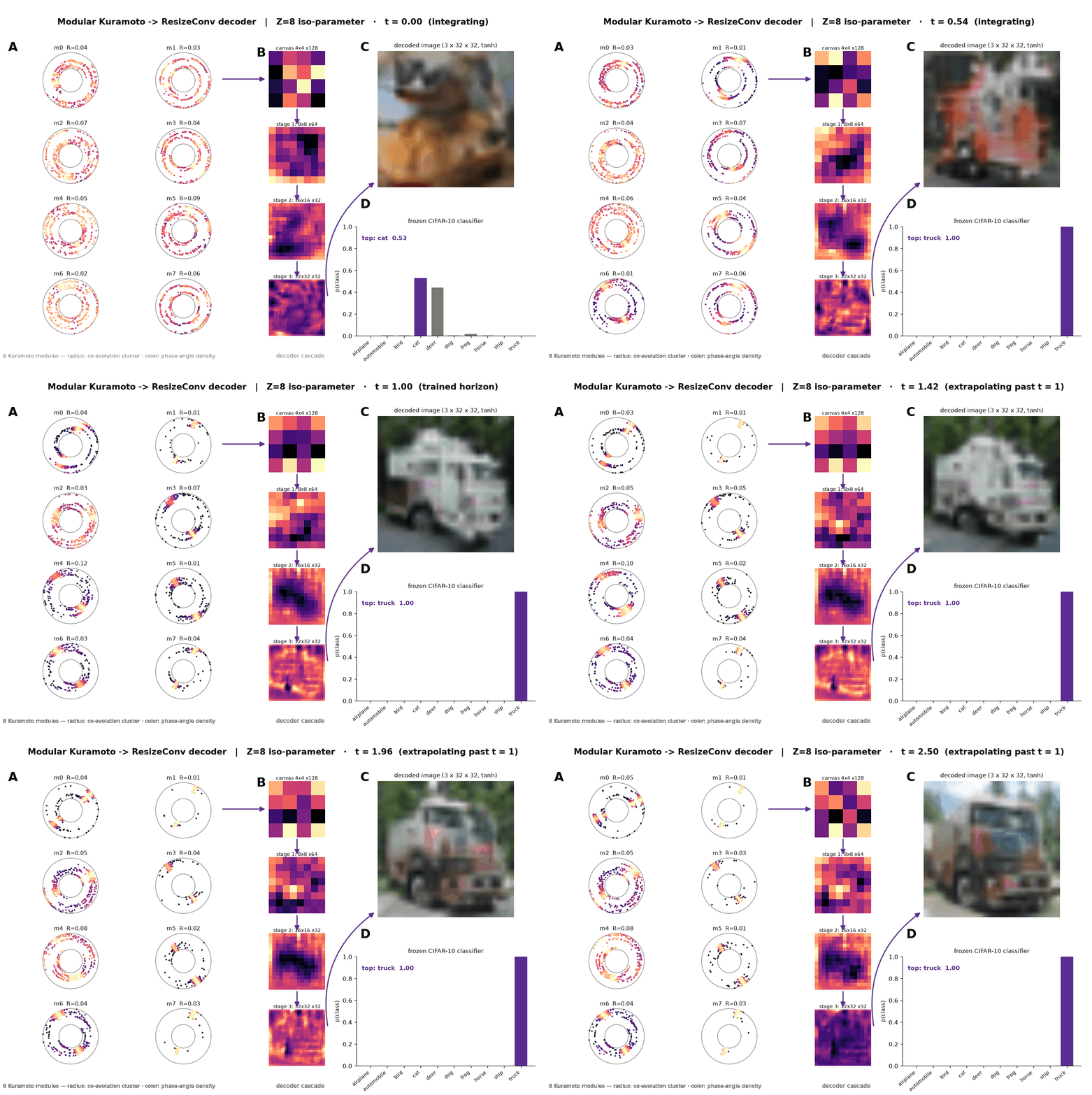 Figure 7: Watching the dynamics of the modular checkpoint. A) The dynamics of the 8x modules of oscillators evolve through time and are read out by our decoder (see B) to generate a resulting image (see C) from a conditioning class and a random initial condition. D) The output image is fed through an offline-trained classifier to return probability of the image’s class. The reader may note that different modules have distinct dynamics.
Each module visualization places each oscillator on a ring and maps oscillator phase to angle — brightness captures share of oscillators at a given phase. We observe the modules are diverse in their dynamics. Some modules anti-phase synchronize into two clusters (e.g., module m1), and others maintain a wide spread of phase angles (e.g., module m4). The dynamics are fast initially and slow down after T=1.
These phenomena are reminiscent of chimera states in classical oscillator systems (Kuramoto & Battogtokh, 2002; Abrams & Strogatz 2004) and modular connectivity organizes a network’s dynamics into a hierarchy of coexisting regimes in tuned dynamical systems (Litwin-Kumar & Doiron, 2012; Kuśmierz et al., 2025).
Patching the modules. We next probe the modular architecture with activation patching to intuit what individual modules are doing. We hot-swap in individual oscillator modules from a horse generation run (B) into an automobile generation run (A), creating a hybrid run, to investigate how individual modules affect the generated image. The following visualization shows the automobile (top-left) and horse (top-right) from the original runs, the hybrid run (top-center), the class of the hybrid run (bottom-right), and weights applied to the hot-swapped horse modules (bottom-center).
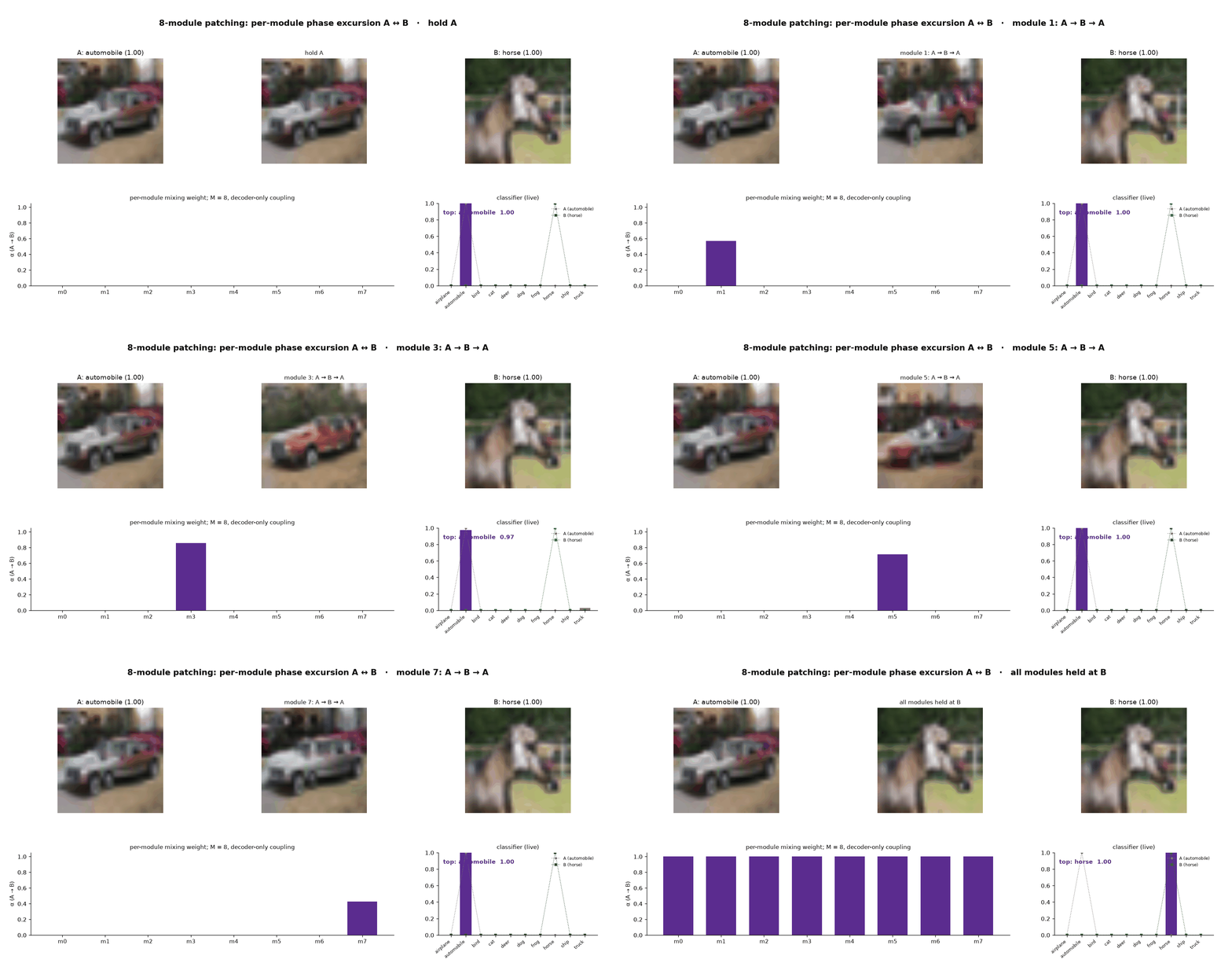 Figure 8: Modules specialize through training. We take two samples from our Z=8 checkpoint of Modular Un-0.1024 (iso-parameter) and interpolate the module phase field on a module-by-module basis from Sample A to Sample B. As we perturb the modules we can see specialized behavior localized to each module. For example, modules m3 and m6 control the color of the car, m7 controls the background color, and m1 appears to reorient the car.
We find modules have distinct functions in this task. Some modules appear to target background (e.g., module m7), others target car orientation (e.g., module m1), and others yet control vehicle color (e.g., modules m3 and m6). The localization of schematic control to individual modules is similar to the learned decomposition of features in β-VAEs (Higgins et al., 2017), multi-pathway networks (Shi et al., 2022), and multi-compartment mechanisms (Goyal et al., 2021).
5. A Systematic Study of Sparsity and Modularity with MNIST1D Classification
We next more deeply study the effect of modularity and sparsity on model performance with a smaller MNIST1D classification task. This task both has a different shape than generative modeling (classification vs generative modeling) and is small enough for extensive hyperparameter tuning and configuration sweeps to be performed. This architecture is composed of fixed-size linear encoders and decoders and a pool of N oscillators:
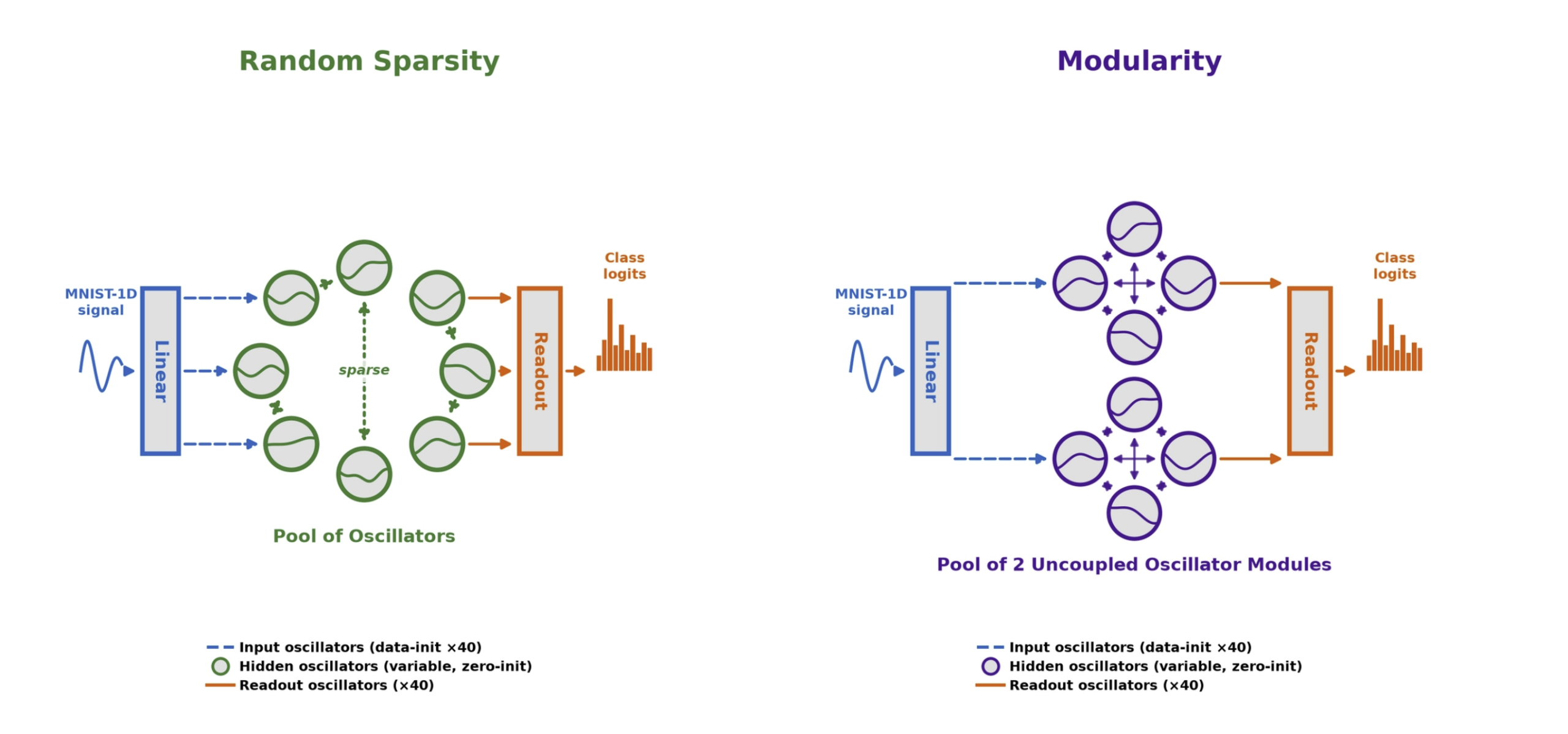
We then hyperparameter sweep many sparsity and size combinations to explore the interplay between validation accuracy, parameter count, and oscillator count. In these experiments, Z=2-40 modules are evaluated for modular sparsity, and s=0.25-0.998 sparsity levels are evaluated for random sparsity. In the below plot, each line is an iso-state experiment with increasing sparsity (blue to red) starting from a dense configuration (dark blue). The x-value is the oscillator count, and the y-value is the validation accuracy. Arcing trajectories indicate that the best accuracy is achieved at moderate sparsity.
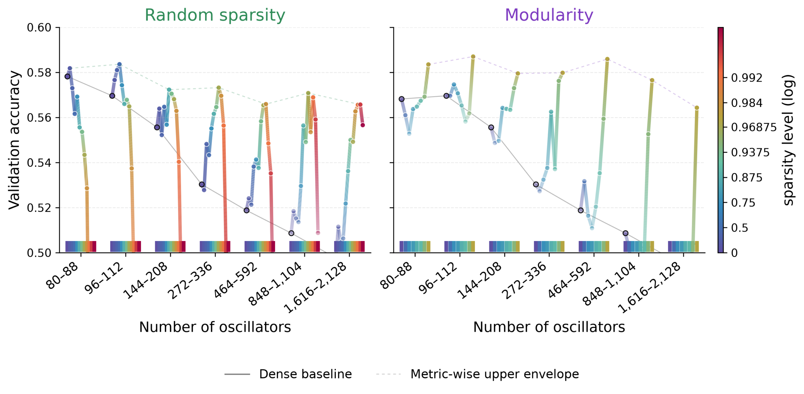 Figure 9: Both forms of sparsity improve over dense in sequence classification MNIST1D with more pronounced benefit at larger system scale. For each size system, we sweep the sparsity represented by color and small offset. Random sparsity (left) illustrates an optimal sparsity level (highest validation accuracy) which scales with system size: larger systems benefit from more sparsity. Modularity (right) benefits from more modules (more sparsity) up until the failure of input being disconnected from the output (data not represented above this threshold).
Dense models struggle to scale, but sparsity in both forms recovers and exceeds performance for an optimal sparsity. Many sparse configurations with different oscillator parameter ratios achieve the same validation accuracy, indicating that sparsity can be negotiated to trade off state variable and parameter count at iso-accuracy. In random sparsity, validation accuracy drops at very low parameter counts (and high sparsity) because input embedding dimensions become disconnected from the output embeddings. We do not study the corresponding regime in modularity due to the abrupt transition where input becomes decoupled from output at high modularity (Z>40).
For configurations with large numbers of state variables, the sparser architectures achieve higher accuracy. We attribute this to sparsity improving the trainability of the model architecture, as discussed below.
6. Why does Sparsity Work?
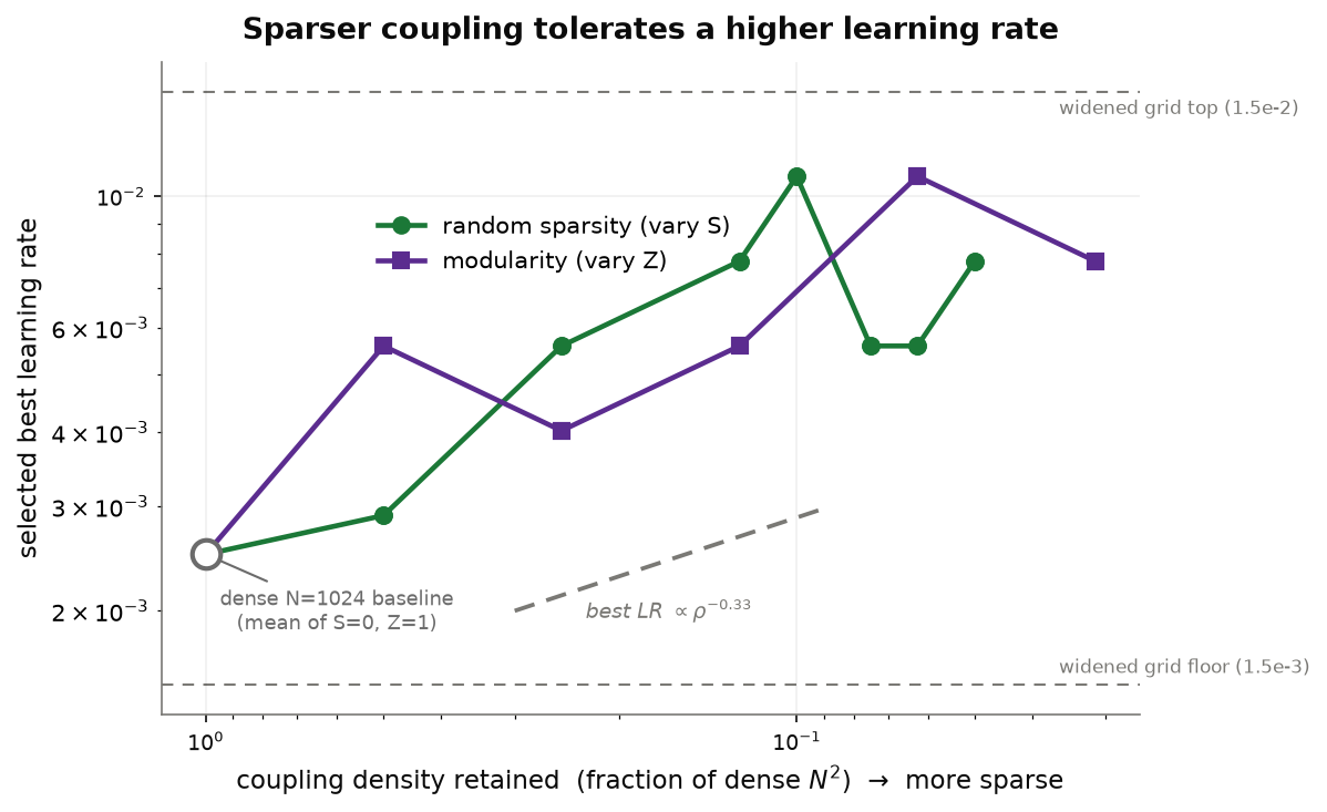
Figure 10: CIFAR-10: more sparse coupling tolerates a higher learning rate before synchronization induced collapse of dimensionality.
Crucially, sparse and modular systems tolerate higher learning rates (LR) indicating greater stability and less hyperparameter sensitivity. Dense models easily fall into catastrophic synchronization into a globally locked, zero-gradient state. Sparsity breaks this all-to-all coupling, allowing the network to maintain high-dimensional dynamics via chimera-like states (coexisting coherent and incoherent activity) and preserving the dimensionality of the dynamics even as the system scales up.
Empirically, the optimal LR scales with sparsity s as \eta^\star \sim (1-s)^{-1/3}. This is shallower than the theoretical expectations from update-to-initialization ratios. This shallow scaling is consistent with two observations: 1) updates are only partially coherent and 2) decoder fan-in remains constant even as we scale system size.
7. Sparse architectures improve recall
Introducing Un-0 suggested a useful working picture for this hybrid generator: the oscillator dynamics organize and preserve the distribution of latent states, while the conventional decoder turns those states into recognizable pixels. If so, changing coupling density should appear most directly in recall. Dense coupling may pull many initial conditions toward the same few dynamical outcomes; sparse coupling may preserve more distinct ones.
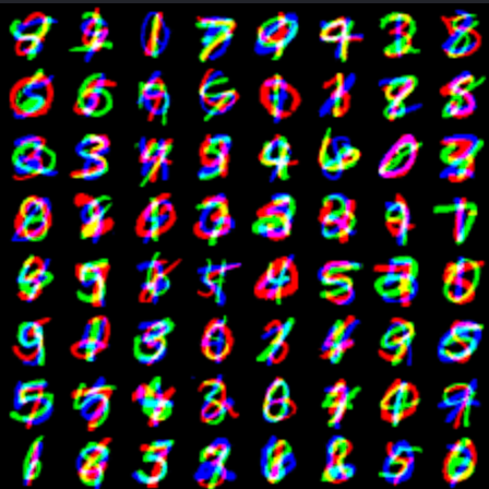 Figure 11: Stacked MNIST example image.
We test this idea with the standard Stacked MNIST benchmark (Metz et al., 2017), where diversity is unusually transparent. Each image combines three independently chosen MNIST digits, one per color channel, yielding 1,000 possible semantic modes. A fixed classifier assigns generated images to these modes, subject to a confidence threshold. In this experimental setup, precision and recall are quantified as follows; refer to Appendix for detailed description of metrics:
- Precision – does the generated image cleanly decompose into three MNIST digits? This is quantified with the manifold precision metric, where higher is better.
- Recall/Diversity – how many combinations of stacked MNIST digits is the model able to generate? This is quantified with effective mode count, where higher is better.
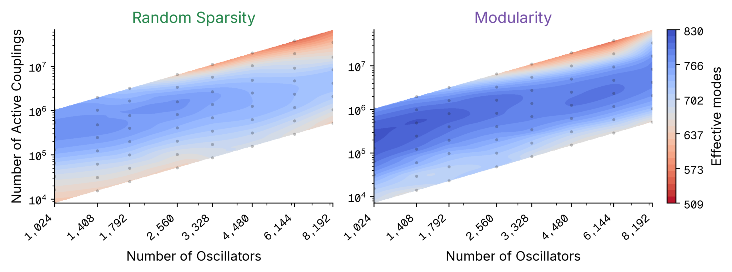 Figure 12: Sparsity enables more diverse samples when comparing across fixed decoders. Stacked MNIST probes for diversity of the images generated using a metric of effective mode count. Dense coupling at large system size shows a significant loss of the effective mode count which both forms of sparsity recover.
The resulting surfaces show a broad high-diversity operating band. Large, strongly coupled systems (upper right) lose diversity: their generated distributions concentrate on fewer modes. Removing connections or dividing the dynamics into modules restores broader coverage. However, sparsity is not universally beneficial: small systems, especially highly fragmented modular ones, can lose performance when interaction becomes too limited. Connectivity therefore acts as a control knob, not a monotonic regularizer.
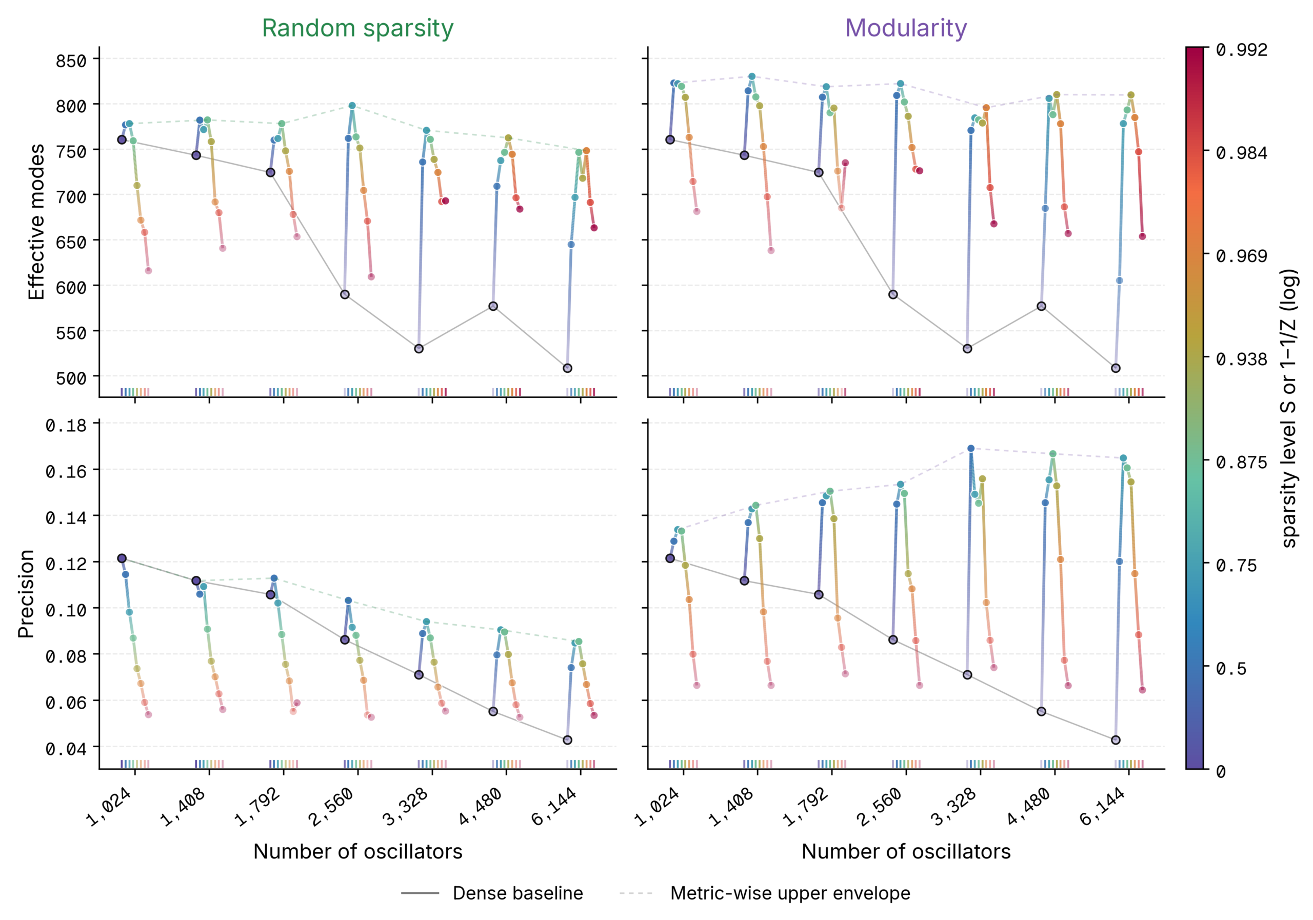 Figure 13: Precision and diversity across system size and sparsity. Labeled x-axis ticks denote oscillator count; colored mini-ticks encode increasing sparsity from purple to red. Solid black lines show dense baselines, while dashed lines trace the upper envelope.
Figure 13 shows precision/diversity across different system sizes and levels of sparsity for both modular and random sparse networks. In the above experiment, the densely coupled baseline degrades in both diversity and precision as system size increases. Across system sizes, moderate sparsity often exceeds the dense baseline in both precision and effective modes; random sparsity is an exception at the two smallest sizes, where it improves effective modes but not precision. The optimal sparsity level still depends on system size and topology. At very high levels of sparsity (red points), a degradation in precision is observed, but recall can remain relatively high — especially for random sparse networks. We suspect that diversity plays a significant role in the observed FID improvements for the generative tasks. For the CIFAR generation experiments, we have found that the FID improvements correlate more closely with recall (correlation=0.924) versus precision (correlation=-0.114), for example.
8. Conclusions and future work
We have shown that sparsity is not simply a powerful tool for driving efficiency of implementation, but also a tool for shaping the trainability and dynamics of unconventional dynamical systems, such as Kuramoto. This work advances this important discussion on our open-source model variant, Un-0, through a direct demonstration of two minimal architectural choices that drive measurable performance gains. Sparsity can fundamentally alter the scaling of unconventional model classes: what sparsity variants will you contribute to this growing community?
References
Abrams, D.M., Strogatz, S.H., (2004). Chimera States for Coupled Oscillators. Phys. Rev. Lett. 93, 174102. https://doi.org/10.1103/PhysRevLett.93.174102
Achterberg, J., Akarca, D., Strouse, D.J., Duncan, J., Astle, D.E., (2023). Spatially embedded recurrent neural networks reveal widespread links between structural and functional neuroscience findings. Nat Mach Intell 5, 1369–1381. https://doi.org/10.1038/s42256-023-00748-9
Bellec, G., Kappel, D., Maass, W., Legenstein, R., (2018). Deep Rewiring: Training very sparse deep networks. https://doi.org/10.48550/arXiv.1711.05136
Breakspear, M., Heitmann, S., Daffertshofer, A., (2010). Generative Models of Cortical Oscillations: Neurobiological Implications of the Kuramoto Model. Front. Hum. Neurosci. 4. https://doi.org/10.3389/fnhum.2010.00190
Caranzano, I., Pancotti, C., Rollo, C., Sartori, F., Liò, P., Fariselli, P., Sanavia, T., (2025). Sparsity is All You Need: Rethinking Biological Pathway-Informed Approaches in Deep Learning. https://doi.org/10.48550/arXiv.2505.04300
Chen, X., Cheng, Y., Wang, S., Gan, Z., Liu, J., Wang, Z., (2021). The Elastic Lottery Ticket Hypothesis, in: Advances in Neural Information Processing Systems. Curran Associates, Inc., pp. 26609–26621.
Frankle, J., Carbin, M., (2019). The Lottery Ticket Hypothesis: Finding Sparse, Trainable Neural Networks. https://doi.org/10.48550/arXiv.1803.03635
Frantar, E., Alistarh, D., (2023). SparseGPT: Massive Language Models Can be Accurately Pruned in One-Shot, in: Proceedings of the 40th International Conference on Machine Learning. Presented at the International Conference on Machine Learning, PMLR, pp. 10323–10337.
Gadhikar, A., Jacobs, T., Zhou, C., Burkholz, R., (2025). Sign-In to the Lottery: Reparameterizing Sparse Training. Presented at the The Thirty-ninth Annual Conference on Neural Information Processing Systems.
Goyal, A., Lamb, A., Hoffmann, J., Sodhani, S., Levine, S., Bengio, Y., Schölkopf, B., (2020). Recurrent Independent Mechanisms. https://doi.org/10.48550/arXiv.1909.10893
Gray, S., Radford, A., Kingma, D.P., (2017). GPU Kernels for Block-Sparse Weights. Block-sparse GPU kernels. OpenAI. URL https://openai.com/index/block-sparse-gpu-kernels/ (accessed 8.6.26).
Han, S., Mao, H., Dally, W.J., (2015). Deep Compression: Compressing Deep Neural Networks with Pruning, Trained Quantization and Huffman Coding arXiv.org. URL https://arxiv.org/abs/1510.00149v5
Higgins, I., Matthey, L., Pal, A., Burgess, C., Glorot, X., Botvinick, M., Mohamed, S., Lerchner, A., (2017). beta-VAE: Learning Basic Visual Concepts with a Constrained Variational Framework. Presented at the International Conference on Learning Representations.
Hizanidis, J., Kouvaris, N.E., Zamora-López, G., Díaz-Guilera, A., Antonopoulos, C.G., (2016). Chimera-like States in Modular Neural Networks. Sci Rep 6, 19845. https://doi.org/10.1038/srep19845
Kozachkov, L., Ennis, M., Slotine, J.-J., 2023). RNNs of RNNs: Recursive Construction of Stable Assemblies of Recurrent Neural Networks. https://doi.org/10.48550/arXiv.2106.08928
Kuramoto, Y., Battogtokh, D., (2002). Coexistence of Coherence and Incoherence in Nonlocally Coupled Phase Oscillators. https://doi.org/10.48550/arXiv.cond-mat/0210694
Kuśmierz, Ł., Pereira-Obilinovic, U., Lu, Z., Mastrovito, D., Mihalas, S., (2025). Hierarchy of Chaotic Dynamics in Random Modular Networks. Phys. Rev. Lett. 134, 148402. https://doi.org/10.1103/PhysRevLett.134.148402
LeCun, Y., Denker, J., Solla, S., (1989). Optimal Brain Damage, in: Advances in Neural Information Processing Systems.
Liebenwein, L., Hasani, R., Amini, A., Rus, D., (2021). Sparse Flows: Pruning Continuous-depth Models arXiv.org. URL https://arxiv.org/abs/2106.12718v2.
Litwin-Kumar, A., Doiron, B., (2012). Slow dynamics and high variability in balanced cortical networks with clustered connections. Nat Neurosci 15, 1498–1505. https://doi.org/10.1038/nn.3220
Liu, S., Mocanu, D.C., Pei, Y., Pechenizkiy, M., (2021). Selfish Sparse RNN Training, in: Proceedings of the 38th International Conference on Machine Learning. Presented at the International Conference on Machine Learning, PMLR, pp. 6893–6904.
Nowak, A.I., Gniecki, Ł., Szatkowski, F., Tabor, J., (2024). Sparser, Better, Deeper, Stronger: Improving Sparse Training with Exact Orthogonal Initialization. arXiv.org. URL https://arxiv.org/abs/2406.01755v1.
Otsuka, H., Chijiwa, D., Okoshi, Y., Fujiki, D., Takeuchi, S., Motomura, M., (2025). The Strong Lottery Ticket Hypothesis for Multi-Head Attention Mechanisms arXiv.org. URL https://arxiv.org/abs/2511.04217v1.
Pikovsky, A., Rosenblum, M., Kurths, J., (2001). Synchronization: A Universal Concept in Nonlinear Sciences, Cambridge Nonlinear Science Series. Cambridge University Press, Cambridge. https://doi.org/10.1017/CBO9780511755743
Semedo, J.D., Zandvakili, A., Machens, C.K., Yu, B.M., Kohn, A., (2019). Cortical Areas Interact through a Communication Subspace. Neuron 102, 249-259.e4. https://doi.org/10.1016/j.neuron.2019.01.026
Shazeer, N., Mirhoseini, A., Maziarz, K., Davis, A., Le, Q., Hinton, G., Dean, J., (2017). Outrageously Large Neural Networks: The Sparsely-Gated Mixture-of-Experts Layer. https://doi.org/10.48550/arXiv.1701.06538
Shi, J., Shea-Brown, E., Buice, M., (2022). Learning dynamics of deep linear networks with multiple pathways, in: Advances in Neural Information Processing Systems. Curran Associates, Inc., pp. 34064–34076. https://doi.org/10.52202/068431-2469
Strogatz, S.H., (2000). From Kuramoto to Crawford: exploring the onset of synchronization in populations of coupled oscillators. Physica D: Nonlinear Phenomena 143, 1–20. https://doi.org/10.1016/S0167-2789(00)00094-400094-4)
Tanaka, H., Kunin, D., Yamins, D.L.K., Ganguli, S., (2020). Pruning neural networks without any data by iteratively conserving synaptic flow. https://doi.org/10.48550/arXiv.2006.05467
Turcu, D., Abbott, L.F., (2022). Sparse RNNs can support high-capacity classification. PLoS Comput Biol 18, e1010759. https://doi.org/10.1371/journal.pcbi.1010759
Xie, E., Mihalas, S., Kuśmierz, Ł., (2025). Slow Transition to Low-Dimensional Chaos in Heavy-Tailed Recurrent Neural Networks, in: Advances in Neural Information Processing Systems. Curran Associates, Inc., pp. 123006–123042. https://doi.org/10.52202/085713-4102
Yu, H., Edunov, S., Tian, Y., Morcos, A.S., (2020). Playing the lottery with rewards and multiple languages: lottery tickets in RL and NLP. https://doi.org/10.48550/arXiv.1906.02768
Zhang, X.-Y., Tang, C., (2025). Heavy-tailed update distributions arise from information-driven self-organization in nonequilibrium learning. Proceedings of the National Academy of Sciences 122, e2523012122. https://doi.org/10.1073/pnas.2523012122
Appendix
Related work
Sparsity is everywhere in the modern Machine Learning and neuroAI literature. To appropriately scope this topic to the current work, we view this body of research through three primary lenses:
- Topology: Is the sparsity random/unstructured, or is it modular/block-sparse?
- Fabric: Is the underlying substrate of computation feedforward or recurrent?
- Mask Dynamics: Is the sparse mask static from the outset of training, or is it dynamically updated (via pruning and growth) across training iterations?
The answers to these three questions determine the architectural similarity of prior research to our current framework.
Here, we view the extensive literature on sparsity in Machine Learning and neuroAI through the lens of three architectural axes: topology, computational fabric, and mask dynamics. Topologically, unstructured sparsity uncovers robust subnetworks via pruning (LeCun et al., 1989; Han et al., 2015; Frankle & Carbin, 2019; Frantar & Alistarh 2023) or flow conservation (Tanaka et al., 2020), even in state-space models (Shihab et al., 2025). Conversely, modular designs, including Depthwise Separable Convolutions, Mixture of Experts, block sparsity, and N:M sparsity (Gray et al., 2017; Zhou et al., 2021), enhance hardware efficiency, generalization, and interpretability (Goyal et al., 2021; Achterberg et al., 2023; Liu et al., 2024). Regarding the computational fabric, sparse Recurrent Neural Networks (RNNs) offer unique advantages over feedforward networks by compressing continuous state updates into low-dimensional manifolds (Turcu & Abbott, 2022; Xie et al., 2025) and pruning structural topology to isolate functional mechanisms and stabilize dependencies (Liu et al., 2021; Zhang et al., 2023). Finally, mask dynamics dictate whether sparse routing dynamically evolves during training to optimize subnetworks (Evci et al., 2019; Frankle & Carbin, 2019; Gadhikar et al., 2025) or remains static from initialization to lock in efficiency immediately (Nowak et al., 2024; Zhang et al., 2026).
This taxonomy applies directly to the work we present here: a static mask established at initialization operating on a recurrent fabric (Gray et al., 2017; Fruengel, 2025). While existing literature primarily exploits sparsity for computational efficiency, we investigate whether connectivity itself can make unconventional oscillator models simultaneously more scalable and performant.
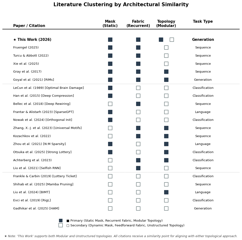 Figure a1: We summarize a subset of the relevant papers using a visual classification based upon the three axes of consideration: 1) the mask dynamics, 2) the architecture of the fabric, and 3) the use of structured/unstructured masks.
Topological Structure: Unstructured vs. Modular Unstructured sparsity, often achieved via Iterated Magnitude Pruning (Frankle & Carbin, 2019) or dynamic flow conservation (Tanaka et al., 2020), uncovers robust subnetworks across diverse architectures, including state-space models like MAMBA (Shihab et al., 2025). Conversely, modular (or structured) sparsity enforces functional isolation and hardware efficiency. Techniques like Depthwise Separable Convolutions (Chollet 2016), Mixture of Experts (MoEs) (Shazeer et al., 2017), block sparsity (Gray et al., 2017), and N:M fine-grained sparsity (Zhou et al., 2021) bypass the memory access inefficiencies of irregular sparse matrices. This modular philosophy actively improves out-of-distribution generalization and mechanistic interpretability, as seen in Brain-Inspired Modular Training (Liu et al., 2024; Achterberg et al., 2023) and Recurrent Independent Mechanisms (Goyal et al., 2021).
The Computational Fabric: Feedforward vs. Recurrent While much of the modern sparsity literature focuses on feedforward networks, applying sparsity to Recurrent Neural Networks (RNNs) yields unique advantages for continuous internal state updates. Sparsely connected RNNs can dynamically support high-capacity processing without dense output units (Turcu & Abbott, 2022). Imbuing recurrent networks with biologically plausible unstructured sparse priors (Xie et al., 2025) forces a slower, robust transition to chaos that compresses representations into efficient, low-dimensional manifolds. Additionally, the structural topology of RNNs can be dynamically pruned, as seen in universal motifs (Zhang et al., 2023) and the Selfish RNN (Liu et al., 2021), to isolate functional mechanisms and stabilize long-term temporal dependencies.
Mask Dynamics: Static Initialization vs. Dynamic Evolution Some methods lean on iterative pruning, others impose static masks. Iterated Magnitude Pruning (Frankle & Carbin, 2019) and continuous adaptation techniques like RigL (Evci et al., 2019) and HAM (Gadhikar et al., 2025) are dynamic methods which actively prune and grow connections during training to uncover highly performant subnetworks. While effective (matching or exceeding dense baselines) they can incur significant overhead. Conversely, static masks fix the sparse topology prior to training. By leveraging carefully constructed initializations—such as orthogonal priors (Nowak et al., 2024) or specific Kolmogorov-Arnold representations (Zhang et al., 2026), static approaches bypass the burden of dynamic pruning, locking in the theoretical and efficiency benefits of sparse routing from the very first forward pass at the risk of choosing a sub-optimal mask.
Alignment with the Current Work By mapping the literature across these axes, we establish a simple yet useful architectural taxonomy. The current work is defined by a static mask established at initialization operating on a recurrent computational fabric. This view overlaps with models like Gray et al. (2017) and Fruengel (2025). The literature asks how to cope with sparsity or exploit it for efficiency. We ask whether connectivity itself can be used to make unconventional oscillator models simultaneously more scalable and more performant.
Methodology CIFAR-10 Generation FID evaluation
We point out the difference in reported baseline between this current work and Un-0.n1024 is attributed to two improvements of our methodology: 1) the use of fully converged adaptive integrators (dopri5) for evaluation, and 2) the use of 25 steps of rk4 integration during training. The first ensures that we are not overfitting to the integration method, and the second balances dynamical system faithfulness with practical training. Importantly, all points on our iso-state and iso-parameter count experiments are subject to the same protocol and comparisons between are internally consistent. We believe that this methodology improves our reporting by overcoming the potential confound of the dynamics of generation overfitting to the integrator of choice.
Methodology for MNIST1D Experiments
Our work on mnist1d classification uses scalable pools of oscillators with fixed encoder and decoder size to compare trainability of oscillator dynamics with more hidden oscillators. To accomplish this we define a stereotypical architecture of 40 input oscillators initialized by a linear encoder, a variable number of hidden oscillators and 40 output decoders. This means that the minimum system size we study is 80 oscillators. The dense architecture scales as P \sim (80+H)^2 + P_{encoder} + P_{decoder}. The decoder and encoder remain unchanged through scaling. These input populations are always disjoint from each other.
The encoder is a linear layer from the MNIST1D data to the initial conditions of our 40 inputs oscillators. The decoder operates on the sine and cosine pairs from the fixed 40 oscillators to define the logits which are then turned to probability with a softmax.
We expand these parameters to the band by integrating two types of sparsity: 1) modularity and 2) random sparsity similar to the sparse Un-0 experiments. Importantly, for modularity (and similar to sparse Un-0) we are careful to ensure an equal number of readout oscillators per module.
For each choice of sparsity and hidden oscillators (S, H), we measure the error (averaged across 5 seeds). Importantly the decoder and the encoder are fixed in size so scaling to higher oscillator counts adds only hidden oscillators. Sweeping sparsity allows us to probe the band of parameters accessible by varying both sparsity and hidden oscillator count. At small system sizes, too much sparsity breaks the graph. At large system sizes, dense coupling causes the system to collapse into low dimensional dynamics (synchronization and anti-phase synchronization) that hurts performance. Sparsity helps avoid this collapse and by extension allows us to scale to larger hidden-state sizes.
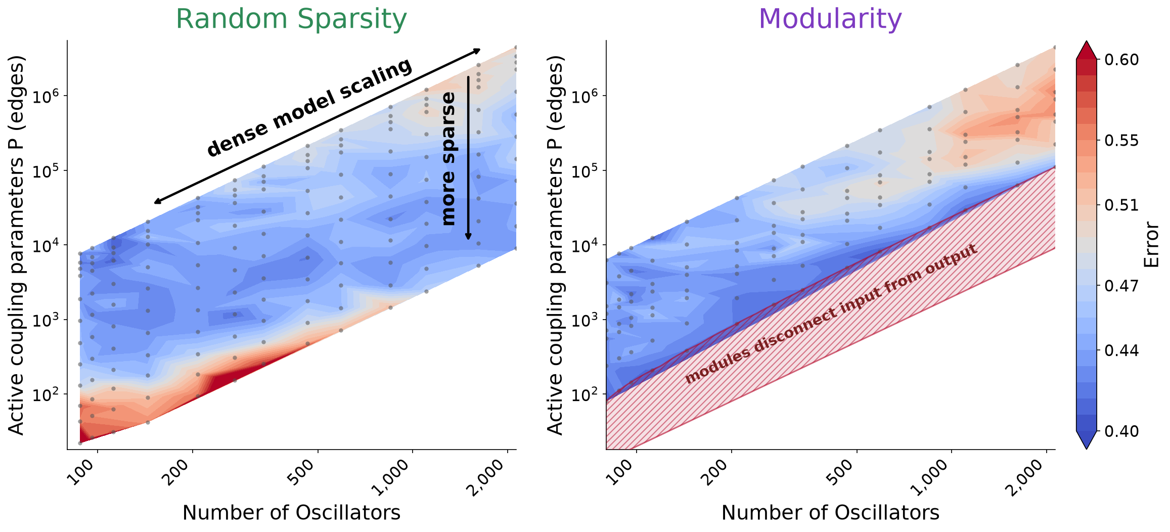
Figure a2: Sparsity of both forms improve our training on simple classification tasks as the number of hidden oscillators in our pool grows. We plot the validation error (5x seeds) on MNIST1D as a colormap over the band of accessible numbers of oscillators versus parameters. The architecture underperforms in two regimes: 1) in the weak communication limit at small active parameters and small numbers of oscillators and 2) in the dense limit of large system size due to synchronization of the oscillator pool.
Complementary to Figure 9, we represent the MNIST1D classification error (1 − validation accuracy) in state size versus parameter count space (see Figure a2). This view corroborates the story in the main text: as system size grows dense models scale poorly, but moderate sparsity can recover and exceed dense performance.
Key Differences between Un-0 and the Sparse MNIST1D Model Architectures
There are two main differences between the classifier and the generative models. The first is the initial condition encoding of the mnist data through a learned linear layer (fixed across scaling). The second is the linear to softmax decoder which maps a fixed number of definitionally disjoint output oscillators to the logits which drive our classification.
Methodology for Stacked MNIST Precision/Diversity Experiments
As in the MNIST1D experiment above, we evaluate paired 8x8 sweeps over system size and connectivity (here over a wider range) while holding the image-facing decoder fixed.
Diversity - Following the Stacked MNIST literature, we first quantify diversity with the reverse KL divergence D_{\mathrm{KL}}\left(p_{\mathrm{gen}}\middle\|u\right) (Metz et al., 2017, Srivastava et al., 2017) from the generated mode distribution p_{gen} to the uniform distribution u over all 1,000 modes (lower is better).
In the main text, we express the same quantity as an effective number of modes. Because u is uniform over 1,000 modes,
D_{\mathrm{KL}}\left(p_{\mathrm{gen}}\middle\|u\right)=\log 1000-H\left(p_{\mathrm{gen}}\right),
and therefore
N_{\mathrm{eff}}=\exp\left(H\left(p_{\mathrm{gen}}\right)\right)=1000e^{-D_{\mathrm{KL}}}.
This is an exact reparameterization of reverse KL, not an additional metric. For example, an effective-mode count of 500 means that the generated distribution has the same entropy as a uniform distribution over 500 modes. It provides an intuitive, continuous, “larger is better” measure of semantic diversity; it is not necessarily the literal number of observed modes.
Precision - To test whether broader coverage merely trades away fidelity, we pair it with an adapted manifold precision metric (Kynkäänniemi et al., 2019). A generated triplet is considered precise when its feature representation lies within a local neighborhood of real examples assigned to the same mode. We construct this manifold in normalized classifier-feature space using Euclidean distance and the k=3 nearest-neighbor rule. The classifier-confidence threshold of 0.8 is used separately when estimating semantic mode diversity.